Capstone: end-to-end research
Every chapter in this series exists to serve one workflow: take an idea, make it concrete, and try as hard as you can to disprove it before a single dollar is at risk. Here we run that workflow start to finish on one strategy — the bare opening-range breakout — from hypothesis, through the backtest, through the full gauntlet, to a verdict. The verdict, as it should be most of the time, is reject. Learning to reach that conclusion cleanly and without regret is the entire point.
Picture the real starting point. You saw the opening-range breakout in a forum thread with a gorgeous equity screenshot, and something in you wants it to be true. That wanting is the adversary, and everything below exists to overrule it. We meet the ORB exactly as you would on a Monday morning — an intuitive idea and a hunch — and then spend the chapter trying to kill it, because the only edge you can trust is one that refused to die. Watch each step as a fresh attempt on its life, and watch the verdict arrive not from opinion but from a number the strategy cannot argue with.
Step 1 — The idea and the hypothesis#
The idea. Markets that break out of their opening range tend to keep going — the first 30 minutes of a session set a reference, and a decisive break of that range is a commitment of order flow that continues into the session. So: buy a break of the range high, sell a break of the low, stop at the opposite edge, target 2R, flatten at the close. One trade per day.
The hypothesis, stated as something falsifiable.The breakout's entry timing captures a real, persistent tendency that pays more than it costs to trade. In expectancy terms we need after costs, and we need it to be distinguishable from what random data would produce. Both halves have to hold. A prior that is merely plausible is not an edge; the job now is to attack it.
Step 2 — Load the data#
Real Nasdaq (US100) M1 bars, restricted to the regular cash session so the "opening range" means what we think it means. ek.data loads and masks the session in two lines.
import edgekit as ek

bars = ek.data.load_bars("US100_M1.csv")
rth  = bars[ek.data.rth_mask(bars.index, start="09:30", end="16:00", tz="America/New_York")]
print(f"{len(bars):,} bars loaded | {len(rth):,} in the regular session")
Step 3 — Build the strategy#
The ORB class is the naive, unfiltered version — no meta-label, no regime gate — which is exactly what you want to stress-test first. The stop sits at the opposite edge of the opening range, so the range width is 1R.
orb = ek.strategy.ORB(or_bars=30, target_r=2.0) # 30-min opening range, 2R targetStep 4 — Backtest and read the metrics#
Run the R-multiple bar loop and summarise with ek.trade_stats. Pass a small intraday warmup and bars_per_day=390 (a 6.5-hour session in minutes).
trades = orb.backtest(rth, warmup=5, bars_per_day=390)
stats  = ek.trade_stats(trades.r, dates=trades.date)
print(f"{stats['n']} trades | win {stats['win_rate']:.0%} | "
      f"PF {stats['pf']:.2f} | EV {stats['ev_r']:+.3f}R")
# -> 2666 trades | win 39% | PF 0.71 | EV -0.214R
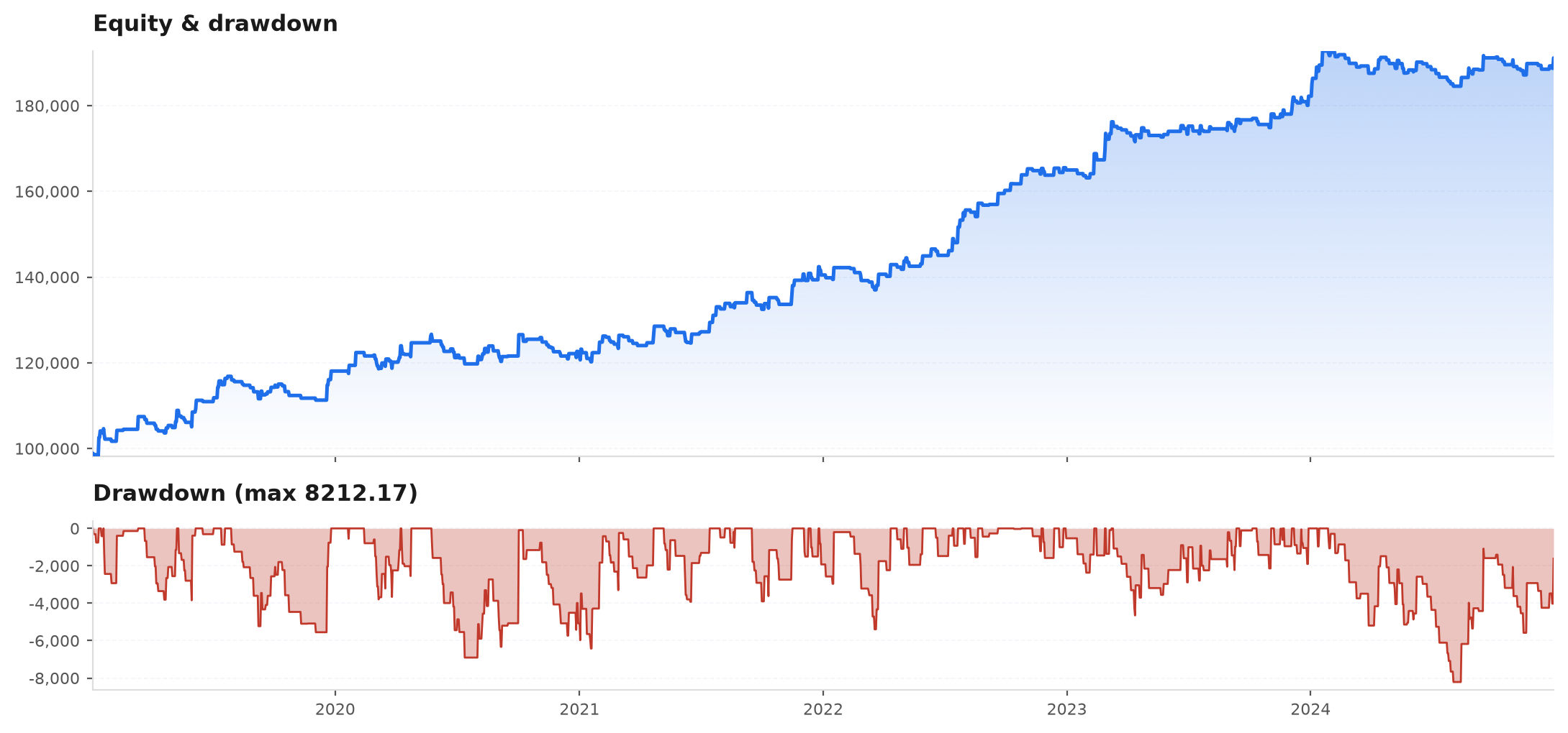
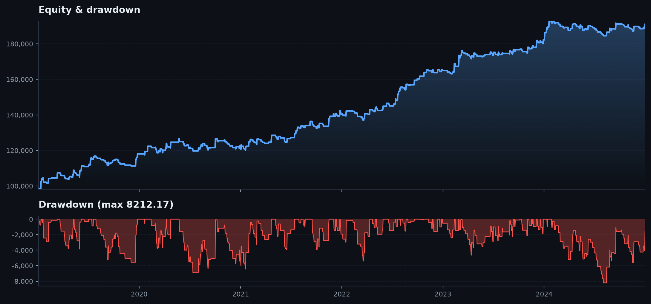
The very first honest number is already damning: is below one, so the strategy loses money net of cost, and expectancy is per trade. With 2,666 trades this is well-powered — not a small-sample fluke. Look at the equity curve and the drawdown together and there is nothing to defend: it grinds down.
Step 5 — Run the gauntlet#
The steps run in order, cheapest-decisive first, and you stop believing at the first failure. See the gauntlet chapter for the full nine-step battery; here are the four that decide this case.
Permutation test — is the timing real?#
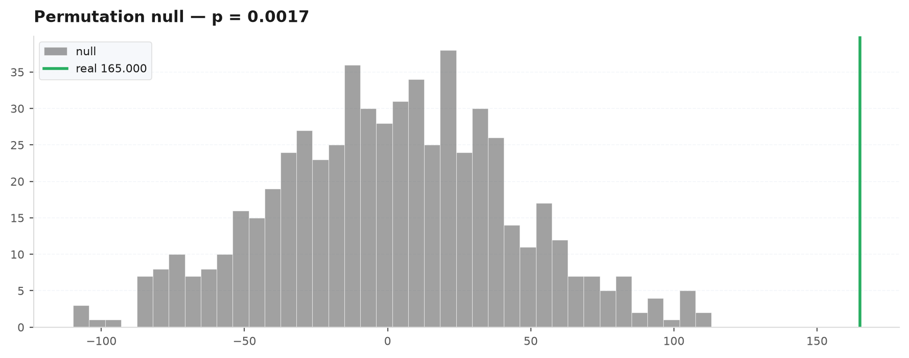
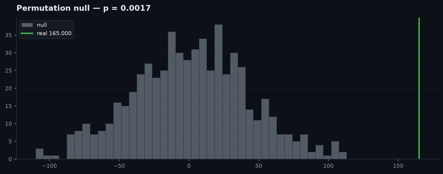
Destroy the market's serial structure while keeping its return distribution exactly, re-run the strategy on each synthetic series, and ask how often random data matches or beats the real total R. The p-value is
import pandas as pd
o, h, l, c = (rth[x].to_numpy(float) for x in ("open", "high", "low", "close"))
idx = rth.index

def null_stat(rng):
    po, ph, pl, pc = ek.validation.permute_ohlc(o, h, l, c, rng)
    sh = pd.DataFrame({"open": po, "high": ph, "low": pl, "close": pc}, index=idx)
    t = orb.backtest(sh, warmup=5, bars_per_day=390)
    return float(t.r.sum()) if len(t) else 0.0

p = ek.validation.mcpt(float(trades.r.sum()), null_stat, n=200)
print(f"permutation p = {p:.3f}")
Here is the subtle, honest result that makes the ORB such a good teaching case: the permutation p is low. On permuted bars the first-touch breakout whipsaws and loses even more, so the real strategy's (still negative) total R sits in the better tail of the null. The entry timing is genuinely non-random. But the permutation test only asks "is the timing structure real?" — it does not ask "does this beat the spread?". Beating a coin flip is not an edge.
Cost stress ×1/2/3 — the decisive gate here#
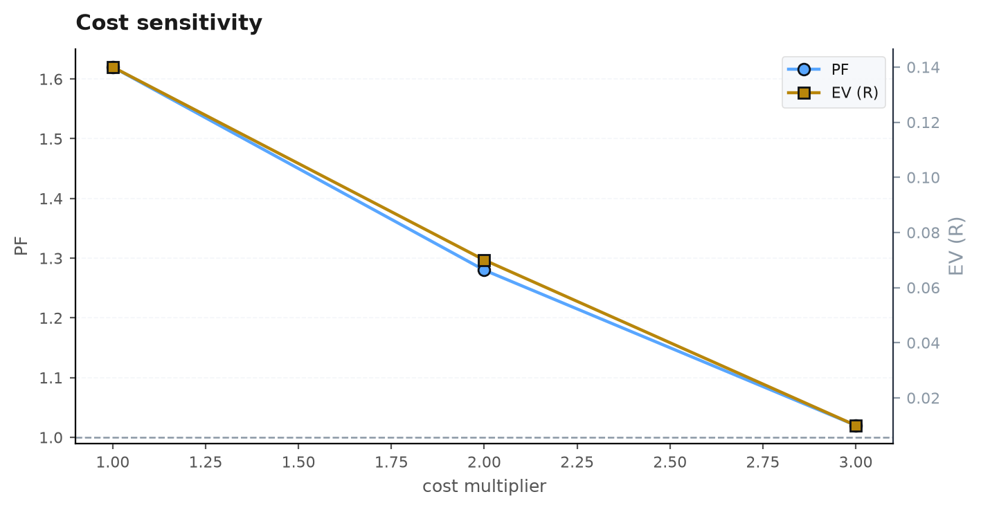
A real edge degrades gracefully as costs rise; a fake one collapses. Re-run at each multiplier.
for m in (1.0, 2.0, 3.0):
    t = orb.backtest(rth, cost=ek.CostModel().scaled(m), warmup=5, bars_per_day=390)
    s = ek.trade_stats(t.r)
    print(f"  {m:.0f}x -> PF {s['pf']:.2f}  EV {s['ev_r']:+.3f}R")
# 1x -> PF 0.71  EV -0.214R
# 2x -> PF 0.45  EV -0.500R
# 3x -> PF 0.29  EV -0.786R
The profit factor never clears 1 — not even at nominal cost — and falls off a cliff as cost escalates. This is the gate the ORB dies at: the faint real tendency the permutation test detected is more than eaten by the transaction cost. The strategy fails the survivor rule (PF > 1 at 2× and 3×) at every level.
Walk-forward — does it hold across regimes?#
A strategy that dies at the cost gate does not earn a walk-forward — but for completeness, the honest sequential-block test asks whether the (net) edge is positive in each consecutive period. A negative-expectancy strategy is unsurprisingly negative in most blocks.
daily = ek.viz.trades_to_daily(trades)                 # net R per calendar day
wf = ek.validation.walk_forward(daily, k=6, refit=False)
print(wf["n_positive"], "of", wf["k"], "blocks positive")
Is it just beta?#
The last false-positive to rule out: is any apparent return really just leveraged exposure to the underlying? Regress the strategy's daily returns on buy-and-hold — beta is the exposure slope, alpha the annualised residual.
bh = rth["close"].resample("1D").last().pct_change().dropna()
out = ek.validation.is_it_beta(daily, bh.reindex(daily.index).fillna(0.0), periods_per_year=252)
print(f"beta {out['beta']:+.2f}  alpha {out['alpha']:+.2%}/yr")
# a negative-expectancy intraday breakout produces no positive alpha to bank
The verdict — REJECT#
Assemble the evidence and the conclusion is unambiguous.
| Gauntlet step | Result | Reading |
|---|---|---|
| Backtest | 2,666 trades, PF 0.71, EV -0.214R | net-negative, well-powered |
| Permutation (step 3) | low p — timing beats random-entry shuffles | structure is real... |
| Cost stress (step 6) | PF 0.71 / 0.45 / 0.29 at 1x/2x/3x | ...but below 1 at every cost — KILLED here |
| Walk-forward / beta | negative across blocks, no bankable alpha | nothing to rescue |
| Verdict | REJECT — never sized, never shipped | the correct, expected outcome |
The ORB clears the first bar (its timing is not pure noise) and fails the second (it does not beat the spread). That distinction — real structure vs. a tradeable edge — is the whole reason the gauntlet exists. We reject the hypothesis, log it, and move on. No sizing, no challenge simulation, no deployment: a negative edge cannot be rescued by dressing it in position-sizing or a portfolio.
If it had survived — sizing and the challenge#
The ORB stops at step 6, so what follows is counterfactual: this is what you would do next only for a strategy whose net edge cleared cost stress, walk-forward, and is-it-beta. Never run these steps on a rejected strategy — a positive-looking sized projection on a negative edge is a lie with a chart.
Size to a drawdown budget#
Size against a block-bootstrapped worst case, not the lucky historical drawdown, then let size_to_dd convert the R-stream into dollars per day under a hard DD budget and a worst-day cap.
import edgekit as ek

daily_r = ek.viz.trades_to_daily(trades)                       # a SURVIVOR's daily R
dd = ek.validation.dd95(daily_r, block=5, horizon=252, n=15000)
sized = ek.sizing.size_to_dd(daily_r, dd_budget=0.095, account=100_000, daily_cap=0.045)
print("$/R", round(sized["dollar_per_r"], 2), "| binding:", sized["binding"])
Simulate the prop-firm challenge#
A prop evaluation is a path problem, so the only honest answer is Monte-Carlo over resampled paths. Feed the sized dollar stream to challenge.simulate.
from edgekit import challenge

rate = challenge.simulate(sized["sized"], challenge.FTMO_1STEP, n=12000)
print(f"pass rate = {rate:.1%}")     # only meaningful for a strategy with a real edge
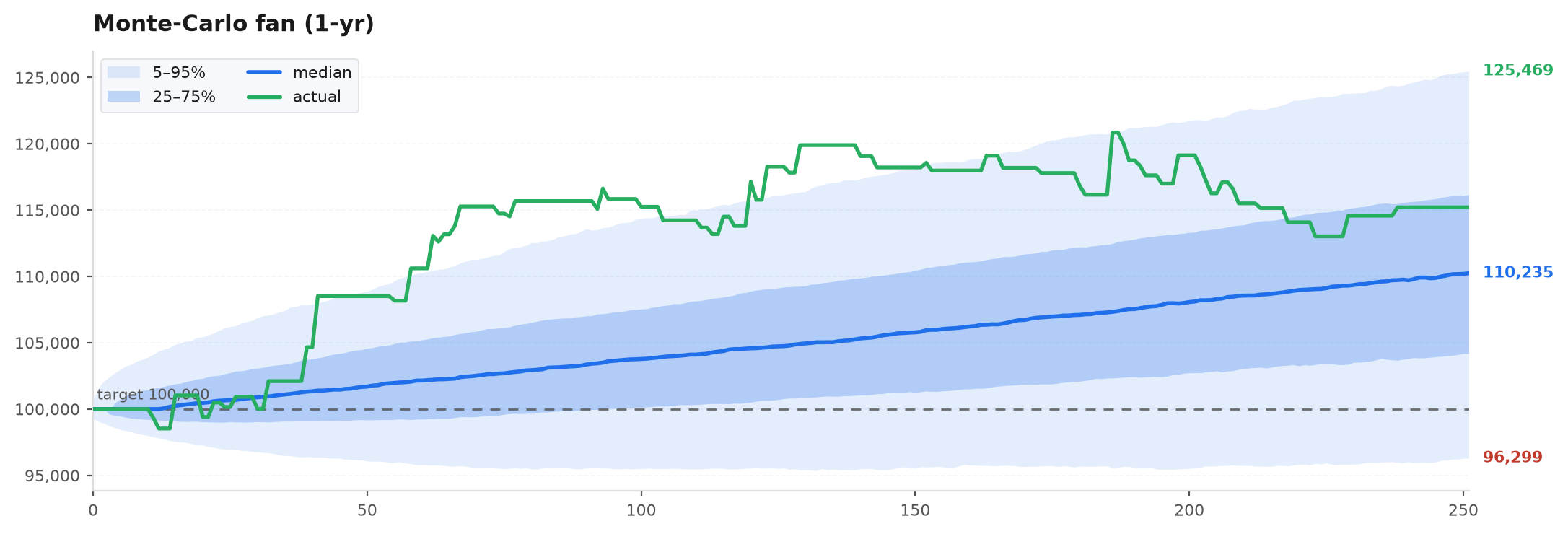
And the forward fan — the same block bootstrap that set dd95 — shows the whole cone of outcomes, so the median (not the backtest ceiling) becomes the planning line. Then, and only then, apply the honest haircut from the previous chapter:
Ship or kill#
The decision is binary and it was made on evidence, not hope:
- Ship only a strategy that survived the whole gauntlet, sized against a bootstrapped worst case, projected with the haircut, paper-reconciled, and monitored with a pre-committed retirement rule (see From backtest to live).
- Kill everything else — which, honestly, is most candidates. The bare ORB is killed at the cost gate. That is not a disappointing result; it is the library doing its actual job.
Where to go next#
You have now seen the full arc — idea, data, strategy, backtest, gauntlet, verdict, and the counterfactual sizing/challenge path a survivor would take. To go deeper:
- API reference — every module and function: data, strategy, metrics, validation, sizing, challenge, ml.
- The validation gauntlet — the nine steps in full, plus the overfit battery (PBO, deflated Sharpe).
- The ORB gauntlet example — this same rejection as a runnable, annotated script.
- Proving an edge — the same tools framed as a how-to for your own candidates.
That is the series. Go build something — then try your hardest to prove it does not work.