The gauntlet

The gauntlet is a fixed, ordered battery whose only purpose is to disprove your strategy. Nine steps, each with one job: try to break the number. Cheap decisive tests come first, expensive ones later, so a strategy that dies at step 3 never earns a walk-forward. This is the tutorial walkthrough; the concept page and API reference have the full detail on each function.

The mindset flip that makes the gauntlet work: you are not the strategy's proud parent, you are its prosecutor. Every step is an attempt to get a conviction — to prove the edge is fake — and the strategy is only "innocent" (worth trading) if it survives every charge you can bring. The order matters because prosecution is expensive: you ask the cheap, decisive questions first (did it read the future? does it survive the spread?) and save the slow ones (walk-forward, bootstrap sizing) for the few candidates that earn them. Most die in the first three steps, and that is the point — the gauntlet's job is to reject, fast.

✕Stop believing at the first failure

The steps are ordered on purpose. When a good number appears, the correct first move is to try to break it — not to celebrate it. What survives all nine is worth sizing; everything else is rejected.

The three ways alpha is fake#

Almost all apparent alpha is one of three things in a strategy costume, and the gauntlet is organised to catch each:

Beta in disguise — the return is just market exposure. Caught by the is-it-beta regression and by permutation (which reshuffles away the drift beta rides on).
Look-ahead — the strategy read the future. Caught first, by construction and property test.
Overfitting — a pattern mined from noise. Caught by permutation, parameter sweeps, PBO, and the deflated Sharpe.

Step 1 — Causality / look-ahead audit#

Checks: every indicator uses prior bars only and every fill is executable. Why first: every later step measures a statistic; if that statistic read the future, everything downstream measures a ghost. In edgekit this is enforced by construction — unlagged indicators, caller lags with ek.lag(x, 1), gap-aware fills — and guarded by a property test that perturbs a future bar and asserts the past does not move.

Step 2 — Realistic fills and costs#

Checks: the P&L survives real spread, slippage, commission, and swap. Why: a gross edge that dies once you pay to trade it is not an edge. edgekit charges cost in R inside the loop via CostModel, so a trade's stored r is already net.

step2_costs.py

import edgekit as ek

cost   = ek.costs.CostModel(spread_rt=0.0012, swap_day=0.0002)   # 12 bps round-trip, 2 bps/day
trades = ek.engine.run_bar_loop(bars, strategy, cost=cost)       # r is net of cost, in R
stats  = ek.trade_stats(trades.r, dates=trades.date)

Step 3 — Monte-Carlo permutation test (the decisive one)#

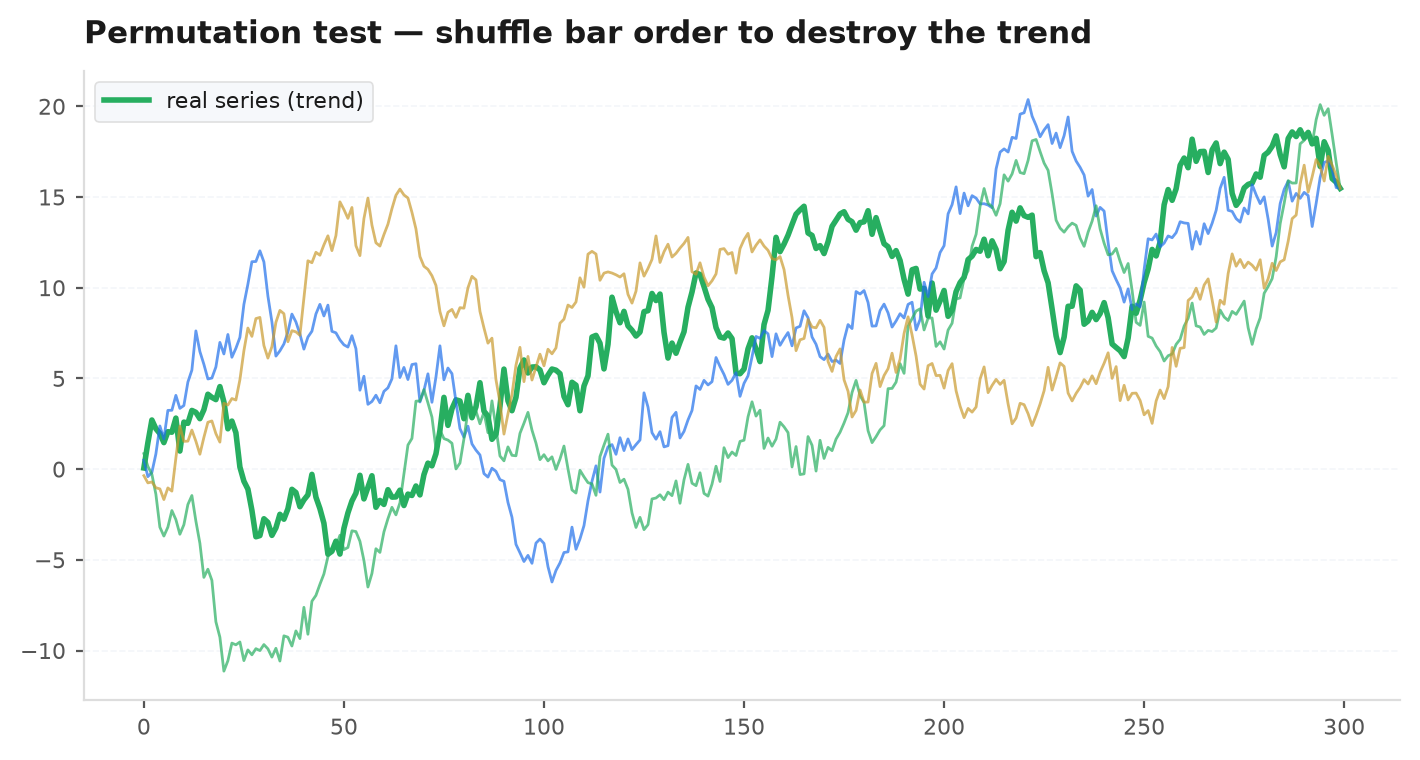
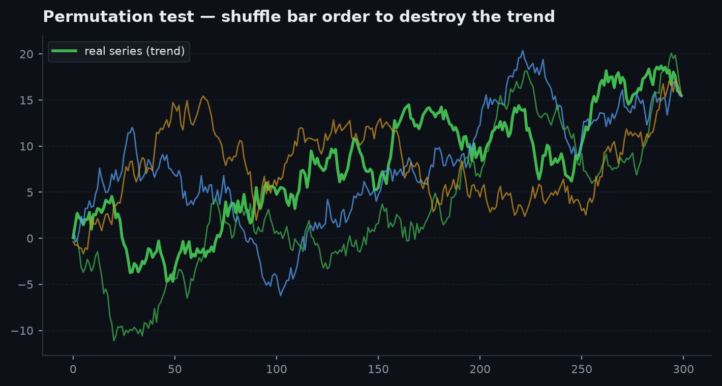
Checks: whether the edge is distinguishable from what random data produces. Why: this is the test edgekit treats as decisive. Destroy the market's structure — the trends and serial correlation a strategy feeds on — while keeping its return distribution exactly, re-run the strategy on many such synthetic series, and ask how often random data matched or beat the real result.

p = \frac{1 + # { s _{i}^{*} \geq s }}{N + 1}

The $+ 1$ counts the observed sample as one of its own permutations, so $p > 0$ always. A no-edge strategy yields $p \sim U (0, 1)$ ; $p < 0.01$ means real. This gets its own long chapter — Monte Carlo.

Real price path beside a structure-destroyed permuted path with the same return marginal — permute_ohlc keeps the return marginal but shuffles the order — the trend the strategy feeds on is gone.

step3_mcpt.py

import edgekit as ek

real = strategy_total_r(bars)
def null_fn(rng):
    po, ph, pl, pc = ek.validation.permute_ohlc(
        bars.open, bars.high, bars.low, bars.close, rng)
    return strategy_total_r(rebuild(po, ph, pl, pc))

p = ek.validation.mcpt(real, null_fn, n=1000)
print(p)     # p < 0.01 -> real edge, not luck

Scenario. Your BTCUSDT breakout earned +64R over the sample. You permute the OHLC bars 1,000 times — each permutation keeps the same set of returns but scrambles their order, killing the trends — and re-run the strategy on each. Only 4 of the 1,000 scrambled markets matched or beat +64R, so $p = (1 + 4) / (1 + 1000) \approx 0.005$ . Verdict: the edge feeds on real serial structure, not the return distribution — it clears the decisive gate. The full step-by-step of this exact calculation is the Monte Carlo chapter.

Step 4 — Walk-forward across regimes#

Checks: the edge persists out-of-sample, sequentially through time — especially in the bad regime. Why: one favourable sample proves nothing; a real edge shows up in block after block.

step4_wf.py

import edgekit as ek

out = ek.validation.walk_forward(daily_r, k=6, refit=False)
print(out["n_positive"], "of", out["k"], "blocks positive")

Full treatment: Walk-forward analysis.

Step 5 — Regime split#

Checks: where the edge earns — across calendar years, and across trend vs chop. Why: a strategy positive in only one year, or one that inverts between regimes, is regime-dependent, not robust.

step5_regime.py

import edgekit as ek

by_year = ek.validation.regime_by_year(trades.r, trades.date)
print(by_year[["n", "ev", "win", "pf", "total_r"]])

adx   = ek.indicators.adx(bars.high, bars.low, bars.close, 14)
split = ek.validation.regime_by_adx(bar_net_r, adx, thr=20.0)
print(split["trend_ev"], split["chop_ev"])

Step 6 — Cost stress ×1/2/3#

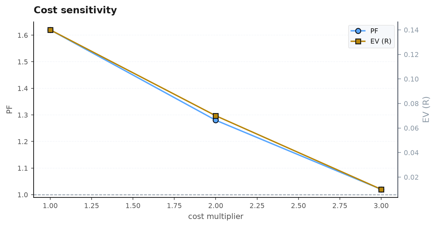
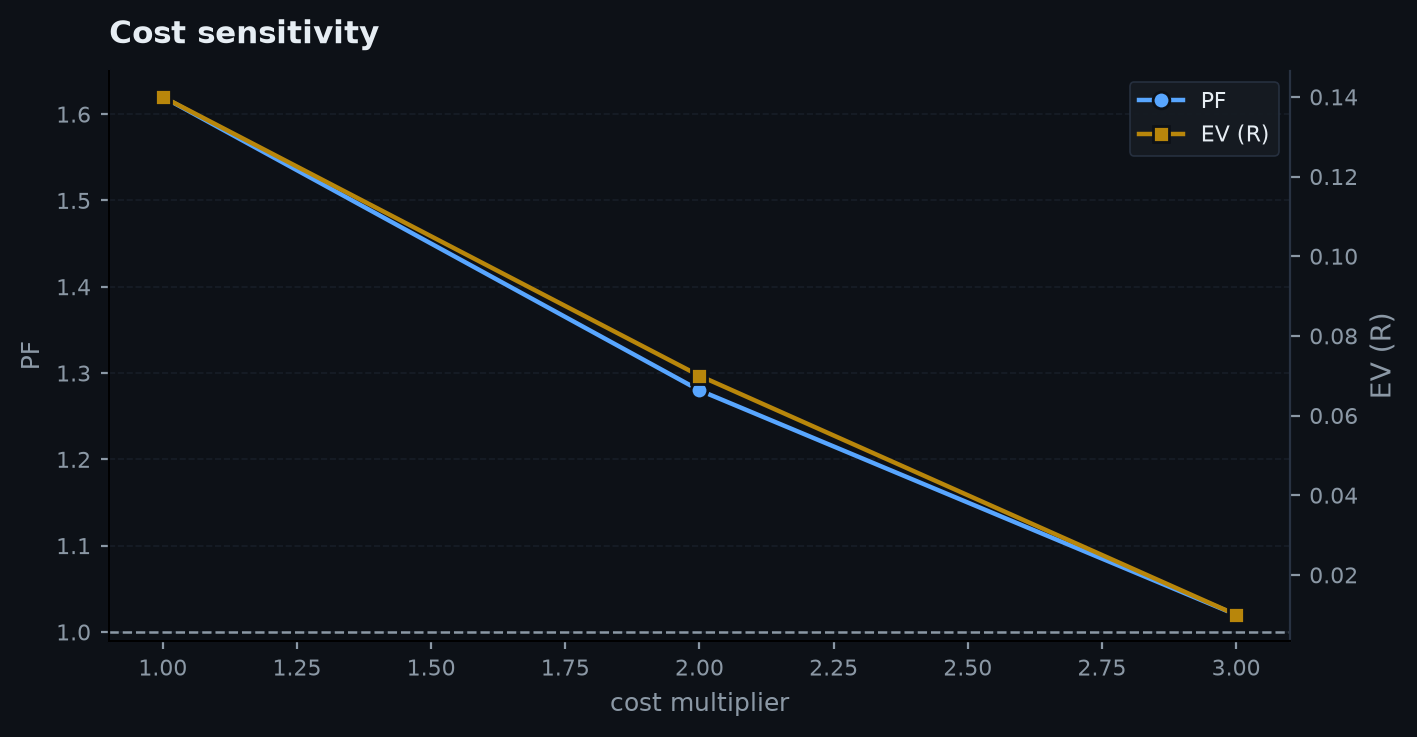
Checks: how the edge behaves as costs escalate. Why: a real edge degrades gracefully; a fake one collapses. Escalating cost is also a proxy for a worse execution environment than the backtest assumed.

Profit factor as a function of the cost multiplier from 1x to 3x — Survivor rule: profit factor must stay above 1 at 2x and 3x. A dip below 1 means the edge lived in the cost assumption.

step6_coststress.py

import edgekit as ek

def run(cost):
    trades = ek.engine.run_bar_loop(bars, strategy, cost=cost)
    return ek.trade_stats(trades.r)

grid = ek.validation.cost_stress(run, base=ek.costs.CostModel(), mults=(1.0, 2.0, 3.0))
for mult, s in grid.items():
    print(mult, "x -> PF", round(s["pf"], 2))     # survivor rule: PF > 1 at 2x and 3x

Step 7 — Is it just beta?#

Checks: whether the return is alpha or leveraged exposure to the benchmark. Why: the classic false positive — a trend follower that is really just long the market shows high beta and ~0 alpha. Regress strategy returns on the benchmark:

r_{s, t} = α + β r_{m, t} + ε_{t}

step7_beta.py

import edgekit as ek

out = ek.validation.is_it_beta(strat_daily_ret, buy_and_hold_daily_ret, periods_per_year=365)
print(out["beta"], out["alpha"])     # want beta near 0 and alpha > 0

Full treatment: Alpha vs beta.

Step 8 — Parameter robustness#

Checks: whether the edge is robust to its knobs. Why: a real effect is a smooth plateau; a knife-edge optimum at one lucky value is overfitting. param_sweep reports the min/median/max spread across a grid.

step8_sweep.py

import edgekit as ek
from edgekit.strategy import ORB

def run(n):
    trades = ek.engine.run_bar_loop(rth, ORB(or_bars=n), warmup=5, bars_per_day=390)
    return ek.trade_stats(trades.r, dates=trades.date)["sharpe"]

sweep = ek.validation.param_sweep(run, grid=range(15, 61, 15))
print(sweep["sharpe_median"], sweep["spread"])   # tight spread = plateau (good)

Full treatment: Overfitting detection.

Step 9 — Honest forward projection#

Checks: the number you can actually trade, not the one that looks best. Why: the drawdown-matched backtest is a ceiling. edgekit never hides the haircut: apply an edge-decay multiplier (≈ ×0.85 if permutation-validated) and a size-down multiplier (≈ ×0.75, because live drawdowns run deeper than the lucky historical one), and size against the block-bootstrap dd95.

step9_forward.py

import edgekit as ek

dd    = ek.validation.dd95(daily_r, block=5, horizon=252, n=15000)   # 95th-pct max DD
sized = ek.sizing.size_to_dd(daily_r, dd_budget=0.095, account=100_000, daily_cap=0.045)
honest = backtest_annual * 0.85 * 0.75      # edge-decay x size-down -> plan around this

The overfit battery#

Alongside the nine steps, two López de Prado diagnostics guard against having tried too many configs: pbo_cscv (want $< 0.35$ ) and deflated_sharpe (want $> 0.95$ ). Both are covered in Overfitting detection.

A worked rejection — the ORB#

The reference recipe runs a bare 30-minute opening-range breakout through the whole battery. It is famous, intuitive, and the gauntlet kills it — which is exactly the point.

Gauntlet step	Result
Trades / result	~2,666 trades, PF 0.71, EV −0.21R — net-negative
Permutation (step 3)	low p — the entry timing beats random-entry shuffles
Cost stress (step 6)	PF `0.71 / 0.45 / 0.29` at 1× / 2× / 3× — below 1 at every level
Verdict	rejected at the cost gate — never sized, never shipped

The honest nuance: the ORB's permutation p is low, so its timing is not pure noise — a real breakout does cluster entries better than a coin flip. And yet its profit factor never clears 1, so it loses money. The permutation test asks "is the structure real?", not "does this beat the spread?". Clearing the first bar and failing the second is the most common story there is, and telling the two apart is the whole job of the gauntlet.

Next: Monte Carlo — the centrepiece: bootstrap resampling, the permutation test in full, forward path simulation, confidence cones, and risk of ruin.