From backtest to live

A strategy that survives the gauntlet has earned the right to be projected forward — not to be believed at face value. The backtest is the best case, the ceiling of what the idea could do on the friendliest data it will ever see. This chapter is about the gap between that ceiling and a live account: how to haircut the number honestly, paper-trade and reconcile, monitor whether the live strategy still tracks its backtest, decide when to retire it, and ship it in a shape the market can actually execute.

Think about the last time you planned a road trip. The map says four hours; you tell everyone six. Not because the map lies, but because the map is the best case — no traffic, no rain, no stop for fuel — and you have driven enough real roads to know the best case is not the plan. A backtest is that map: the fastest the strategy could ever have gone, on the one stretch of road it has already seen. This chapter is the discipline of turning the map time into the arrival time you actually promise — haircutting the number, watching the road live, and knowing in advance the point at which you turn around.

✕Never trade a strategy that didn't survive the gauntlet

Everything below assumes the strategy already passed the gauntlet — permutation, cost stress, walk-forward, is-it-beta. Deployment is not a place to relax skepticism; it is where a fake edge costs real money. A backtest that only looks good has no business anywhere near a live account. The bare ORB in these examples would be killed at the cost gate and would never reach this page — treat that as the norm, not the exception.

The backtest is a ceiling, not a forecast#

The drawdown-matched backtest is the most optimistic honest number you have. It was measured on the one historical path that actually happened — a path that, by survivorship, tends to have been kinder than the future will be. Two things systematically erode it, and edgekit never hides either. Apply both, as multipliers, to the sized projection:

Edge decay ≈ ×0.85. Even a permutation-validated edge weakens as other participants arb it away and as the regime drifts to something less favourable than the sample. If the edge was not permutation-validated, the haircut is far steeper — but such a strategy should not be here at all.
Size-down ≈ ×0.75. Live drawdowns run deeper than the single lucky historical one. Size against a block-bootstrapped dd95 (a bad-but-not-tail drawdown), never the realised max, then shade the projection down further.

R_{honest} = R_{backtest} \cdot edge decay 0.85 \cdot size-down 0.75 \approx 0.64 R_{backtest}

Roughly two-thirds of the headline. That is not pessimism; it is the number you can plan a business around. A strategy whose haircut projection is still worth trading is robust; one that only works at the ceiling was never real.

forward.py

import edgekit as ek

# daily_r is the strategy's net-of-cost daily R stream (post-gauntlet)
# 1. size against a realistic worst case, not the one lucky historical drawdown
dd = ek.validation.dd95(daily_r, block=5, horizon=252, n=15000)   # 95th-pct max DD
sized = ek.sizing.size_to_dd(daily_r, dd_budget=0.095, account=100_000, daily_cap=0.045)
dpr = sized["dollar_per_r"]                                        # applied $/R scalar

# 2. annualise the sized backtest, then haircut it
per_year = 252
backtest_annual = dpr * float(daily_r.sum()) / len(daily_r) * per_year   # ceiling
honest_annual   = backtest_annual * 0.85 * 0.75                          # plan around THIS
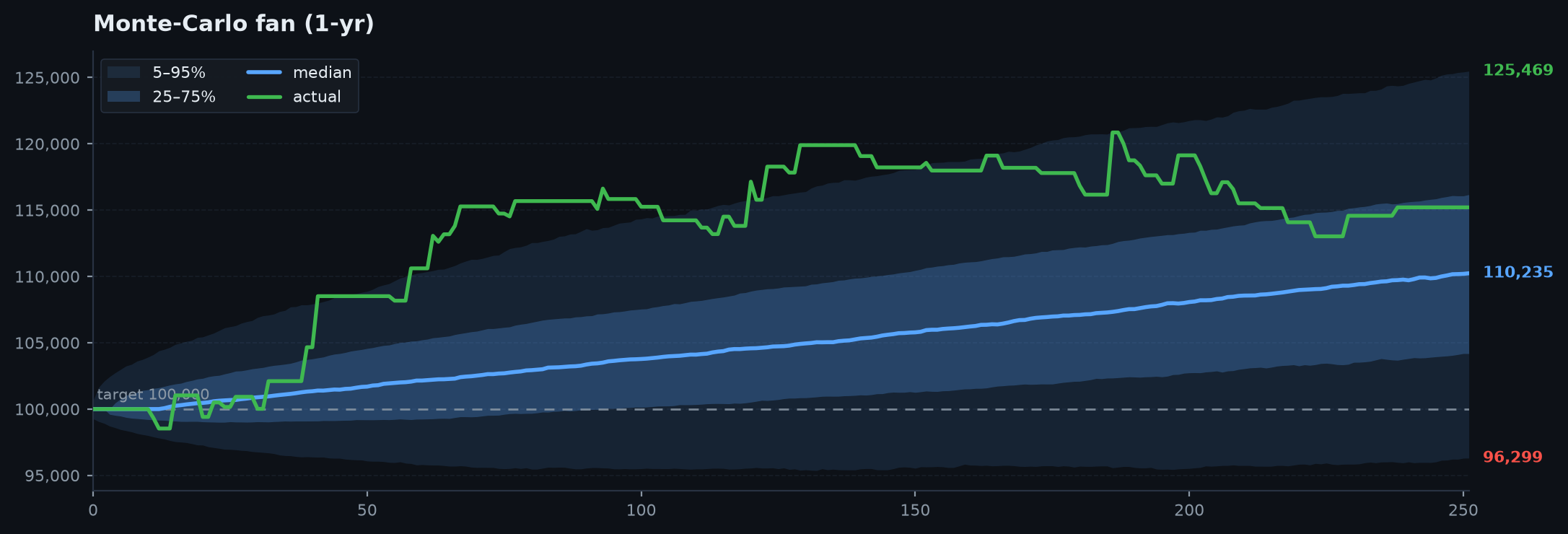
print(f"backtest ${backtest_annual:,.0f}/yr  ->  honest ${honest_annual:,.0f}/yr")

✦Scenario: from a $47k backtest to a $30k plan

A survivor SmaCross book, sized to a 9.5% drawdown budget on a $100k account, backtests at

$47, 000

a year. That is the map time. Apply the two haircuts in turn: edge decay

\times 0.85

takes it to

$40, 000

(other players arb it, the regime drifts), and size-down

\times 0.75

takes it to

$30, 000

(live drawdowns run deeper than the one lucky history, so you carry less size per dollar of budget). You do not put $47k in the business plan — you put $30k, and you treat any live year that lands between $30k and $47k as on-plan. The book that still justifies its capital at $30k is the one worth trading; the one that only works at $47k was a map you mistook for a road.

The forward Monte-Carlo fan makes the ceiling-vs-plan distinction visual. Block-bootstrap the sized daily stream into thousands of forward-year paths and you see the whole cone of outcomes — the median is not the headline, and the lower bands are where risk budgets are actually set.

fan.py

import edgekit as ek, numpy as np
from edgekit import viz

mc = ek.validation.block_bootstrap_mc(daily_r, block=5, horizon=252, n=20000)
print("median terminal", np.median(mc["terminal"]), "| dd95", ek.validation.dd95(daily_r))

# a paths array for the fan (n_sims x horizon) built from the same block bootstrap
fig = viz.mc_fan(paths, actual=daily_r.cumsum().to_numpy(), title="Forward equity — 1y")
viz.save_png(fig, "mc_fan.png")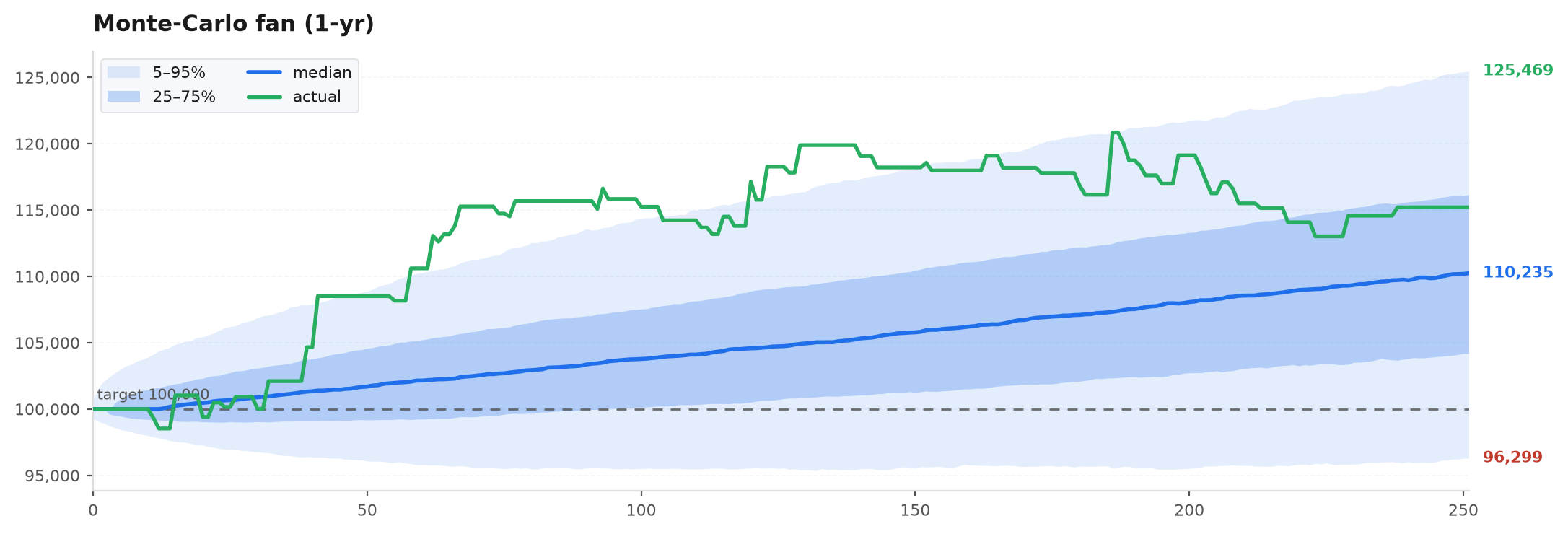

Monte-Carlo fan of forward equity paths — Forward fan from the block bootstrap. The median (not the backtest) is the planning line; the lower bands set the risk budget.

Paper trading and reconciliation#

Before real capital, run the deployed engine on live data and record what it would have done. The point is not more profit evidence — the backtest already gave that — it is a reconciliation: do the live-engine fills, timestamps, and R-multiples match what the backtest produced on the same bars? Any divergence here is a bug (a look-ahead the backtest smuggled in, a timezone or session boundary off by one, a cost model that disagrees) and it is far cheaper to find in paper than in production.

reconcile.py

import edgekit as ek
import numpy as np

# same strategy, same bars: paper engine output vs. the backtest it must reproduce
bt   = ek.trade_stats(backtest_trades.r, dates=backtest_trades.date)
live = ek.trade_stats(paper_trades.r,    dates=paper_trades.date)

for k in ("n", "win_rate", "ev_r", "pf"):
    print(f"{k:9s}  backtest {bt[k]:.3f}   paper {live[k]:.3f}")

# trade-for-trade: on overlapping dates the R-multiples should agree to tolerance
merged = backtest_trades.merge(paper_trades, on="date", suffixes=("_bt", "_live"))
gap = np.abs(merged["r_bt"] - merged["r_live"])
assert gap.max() < 1e-6, f"engine disagrees with backtest by {gap.max():.4g}R — find the bug"

!Reconciliation is a correctness test, not a performance test

If paper trading disagrees with the backtest on the same data, do not average the two and move on. Stop and find why. A mismatch means one of them is wrong, and the backtest — the number you validated — is usually the one that was cheating. See Causality.

Monitoring a live strategy — is it still tracking?#

Once live, the question is continuous: is the strategy behaving like the thing you validated? You do not have the luxury of a large live sample, so you monitor the distribution, not any single trade. The natural statistic is a running expectancy with its standard error. Under the backtest expectancy $μ_{0}$ , the live mean R over $n$ trades has standard error $σ / n$ , so a simple z-score tells you whether live has drifted below plan by more than noise:

z = \frac{R ˉ _{live} - μ _{0}}{σ / n}

A single losing trade means nothing — a strategy that wins 40% of the time loses six in a row roughly once every couple of hundred trades. What matters is whether the live expectancy is consistent with the haircut projection (not the ceiling). Compare live against $μ_{0} = 0.85 \cdot 0.75 \cdot EV_{backtest}$ , not the raw backtest EV, or you will retire good strategies for underperforming a number they were never expected to hit.

monitor.py

import edgekit as ek
import numpy as np

live = ek.trade_stats(live_trades.r)
mu0  = 0.85 * 0.75 * backtest_ev_r          # the PLAN expectancy, not the ceiling
n    = live["n"]
sd   = float(np.std(live_trades.r, ddof=1))
z    = (live["ev_r"] - mu0) / (sd / np.sqrt(n))
print(f"live EV {live['ev_r']:+.3f}R vs plan {mu0:+.3f}R  ->  z = {z:+.2f}")
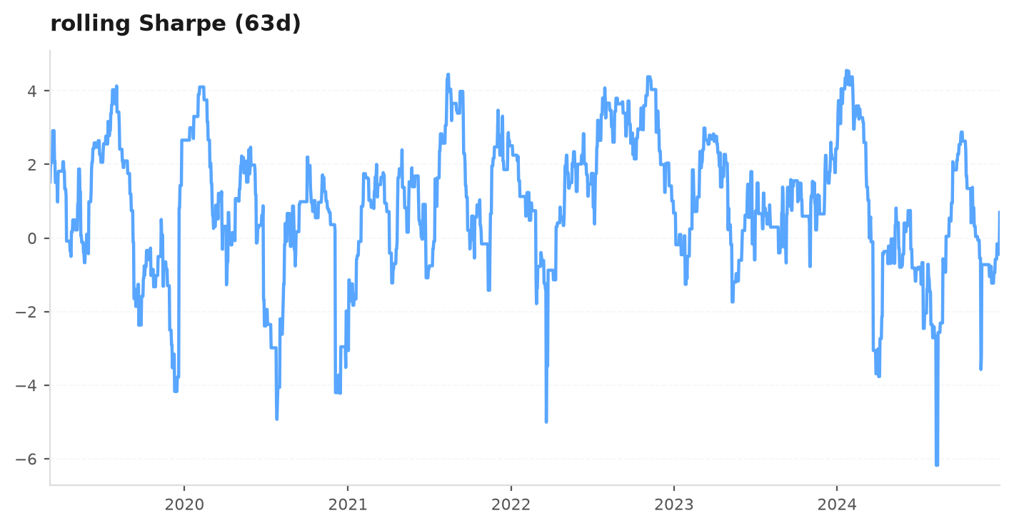
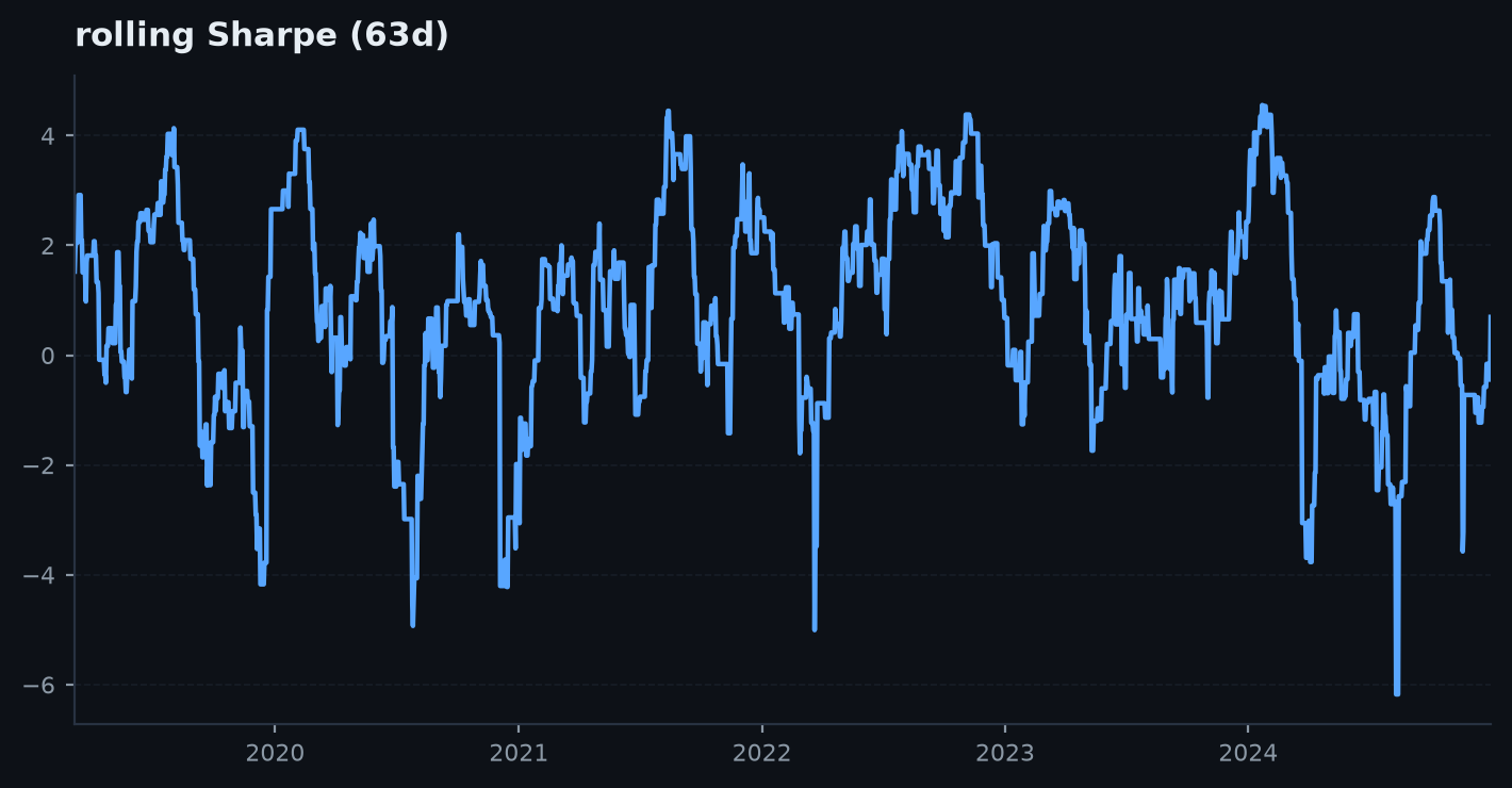
# z near 0: tracking. z << -2 over a meaningful n: investigate, don't panic-close.

✦Scenario: is a -3R week a problem?

Twelve trades into live, your SmaCross book is down 3R and your gut says kill it. Do the arithmetic instead. Plan expectancy is

μ_{0} = 0.85 \times 0.75 \times 0.20 = + 0.13 R

per trade; live is running

R ˉ = - 0.25 R

with a per-trade SD of

σ \approx 1.1

. The z-score is

z = (- 0.25 - 0.13) / (1.1/ 12) \approx - 1.2

— well inside noise; a book this size prints a

- 3 R

stretch routinely. You do nothing. Only when

z

sits below

- 2

across a meaningful n (dozens of trades, not a dozen) is the drift bigger than the streak and worth investigating. The number, not the gut, decides.

Watch the shape of the live equity and its rolling metrics next to the backtest, not just the endpoint. A strategy can end near plan while its character — win rate, average hold, drawdown depth — has quietly shifted, which is the early signature of a changing regime.

Rolling live performance metrics vs backtest baseline — Rolling win rate, expectancy and Sharpe. Tracking is a band around the plan line, not a match to the backtest ceiling.

Edge decay and when to retire#

Edges are not permanent. Crowding, structural market changes, and your own capital moving the market all wear an edge down. The discipline is to decide the retirement rule in advance, so the decision is not made emotionally after a drawdown. Two honest triggers:

Statistical: live expectancy has fallen below the lower bound of its plan for a meaningful sample — the z-score above sits well under −2 across enough trades that it is no longer a streak.
Structural: the drawdown has breached the dd95 you sized against. A live drawdown deeper than the 95th-percentile bootstrap is evidence the return distribution has changed, not merely bad luck within it.

A cumulative-sum (CUSUM) of realised-minus-expected R is a clean way to see decay before the equity curve makes it obvious: it drifts flat while the edge holds and turns persistently down when it fades.

S_{t} = max (0, S_{t - 1} - (R_{t} - μ_{0}))

decay.py

import edgekit as ek
import numpy as np

# CUSUM of shortfall vs plan expectancy — rises when live underperforms plan
r   = live_trades.r.to_numpy(float)
mu0 = 0.85 * 0.75 * backtest_ev_r
S, series = 0.0, []
for rt in r:
    S = max(0.0, S - (rt - mu0)); series.append(S)

# structural trigger: has live DD breached the dd95 we sized against?
worst = ek.validation.dd95(live_daily_r, horizon=252)
print("CUSUM shortfall:", round(series[-1], 2), "| breached dd95:", worst)

✦Scenario: the retirement rule fires

You pre-committed both triggers before going live, so the hard decision is already made when the day comes. Eight months in, the CUSUM shortfall — flat for the first six — starts a persistent climb and crosses the threshold you set, while the live drawdown touches

11%

against a dd95 of

9.5%

. Both triggers agree: the return distribution has changed, not merely dipped. Because the rule was written in advance, you retire the book with no sunk-cost argument running in your head, redeploy the capital to what still survives the gauntlet, and file the corpse in the research log. Six months of earnings, one clean exit — the edge working as designed, then ending on schedule.

✦Retiring a strategy is not a failure

A strategy that earned its keep for two years and then decayed did its job. The failure mode is holding a dead edge out of sunk-cost attachment. Retire on the pre-committed rule, redeploy the capital to what still survives the gauntlet, and keep the corpse in the research log — decayed edges sometimes return in a new regime.

Execution realities vs the backtest#

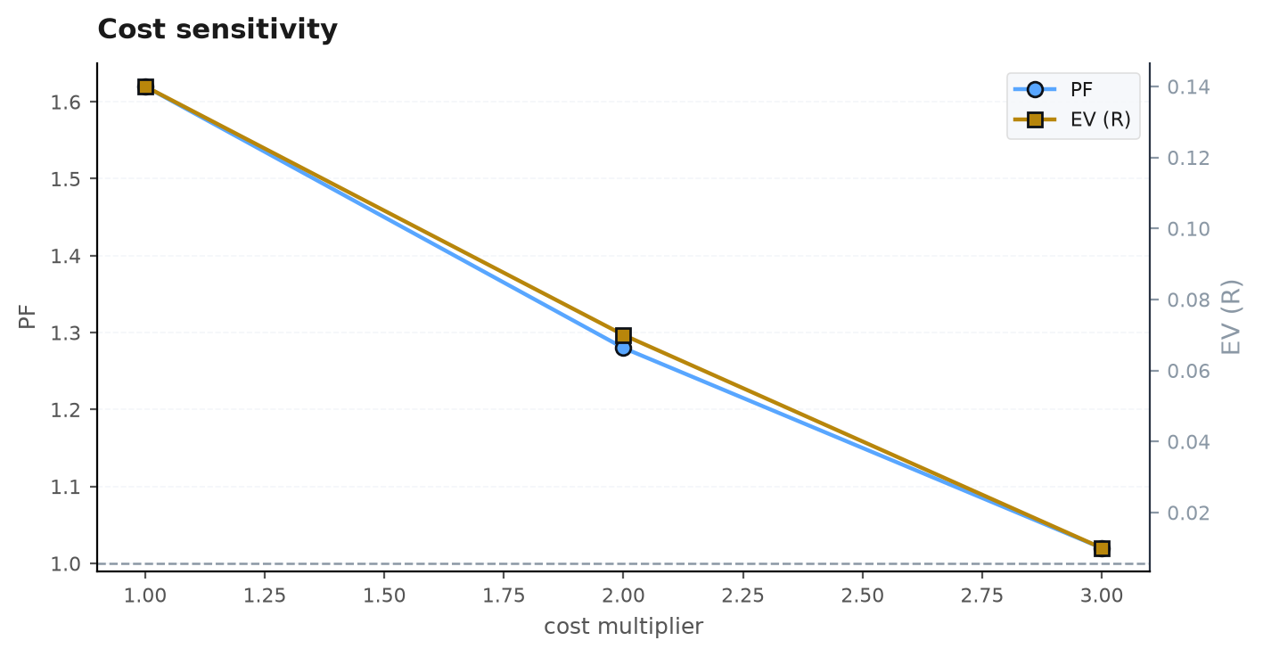
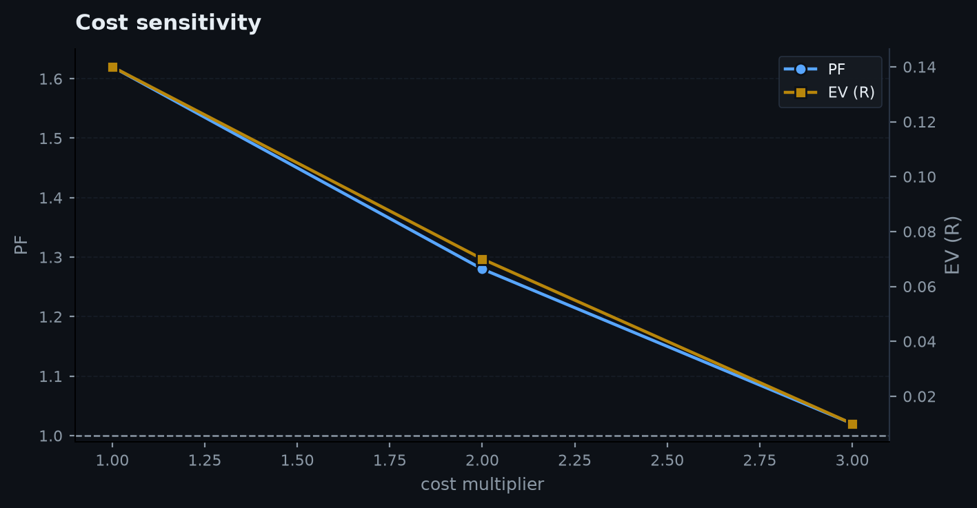
The backtest fills at clean, deterministic prices. Live execution does not, and the gap is a cost the backtest under-charges. This is exactly why cost stress (gauntlet step 6) matters: re-running at 2× and 3× assumed cost is a proxy for a worse execution environment than the backtest assumed. If the edge survives 3× cost, it has headroom for the frictions below; if it dies at 2×, live execution will finish the job.

Reality	What the backtest assumed	Effect on live R	Guard
Slippage	fill at the modelled level/open	each trade a touch worse than modelled	widen spread_rt in CostModel; verify vs paper fills
Latency	instant decision-to-fill	the level you saw is not the level you get	use next-bar-open fills (the engine already does)
Partial fills	full size, always	realised size < intended, R distorted	size below the level that moves the book; reconcile size
Gaps / halts	continuous prices	stops fill past the level (worse than 1R)	gap-aware fills; treat stop-through as a real risk

edgekit charges cost in R through the CostModel, and the bracket engine already imposes the two most important realities: a bar that touches both stop and target counts as the stop, and fills happen at the next bar's open, never on the signal bar. That removes the two biggest live-vs-backtest surprises before you ever deploy. What remains — slippage and partial fills — is what the cost-stress headroom is buying you insurance against.

Scenario. Your US100 ORB stop sits at 18,238. Overnight a headline gaps the open straight to 18,225 — the engine fills your stop at 18,225, not 18,238, so what the backtest booked as $- 1 R$ lands as $- 1.35 R$ live. One gap is noise; a strategy whose backtest is thick with stops in fast, gap-prone conditions is quietly under-charged for exactly this, trade after trade. That structural under-charge is what cost-stress at 2× and 3× stands in for: if the edge still clears PF 1 when you double the assumed cost, it has the headroom to absorb the real gaps and slippage the table above lists.

Profit factor as trading cost is escalated — The cost-stress curve is your execution-reality budget. Only an edge with room above PF 1 at 2-3x cost has headroom for live slippage.

Deployment shapes#

A validated strategy ships as one of two shapes, and the choice is about where the decision logic runs.

A rules engine#

If the strategy is pure rules — indicator crossovers, breakout levels, bracket exits — it deploys as a small deterministic engine that mirrors the backtest loop exactly: read the last closed bar, compute lagged indicators, apply the same entry/exit logic, place a bracket order. Because BaseStrategy already separates prepare / entry / exit from the backtest wiring, the same object that was validated is the specification the live engine implements — no translation gap.

rules_engine.py

import edgekit as ek

strat = ek.strategy.SmaCross(fast=20, slow=100, atr_n=20, stop_mult=2.0)
# the SAME object you validated. Live loop reuses its prepare/entry/exit on closed bars:
#   ind = strat.prepare(bars_so_far)     # indicators are lagged by construction
#   if strat.entry(i, ind): place_bracket(...)   # act only on the last CLOSED bar

Cloud-safe exported models#

If the strategy carries a machine-learning meta-label (a model that decides whether to take an otherwise-triggered signal), you cannot always ship scikit-learn to the execution venue — a broker cBot or a cloud runtime may forbid heavyweight or networked dependencies. ek.ml.export_trees serialises a fitted gradient-boosting classifier to a plain blob, and a pure-Python (or emitted C#) forward pass reproduces predict_proba to float tolerance — no sklearn at runtime.

export.py

import numpy as np
from edgekit.ml import export_trees, tree_predict_proba, MetaLabeler, emit_python

blob = export_trees(clf)                       # fitted HistGradientBoostingClassifier -> str blob
assert np.abs(tree_predict_proba(blob, X) - clf.predict_proba(X)[:, 1]).max() < 1e-6

meta = MetaLabeler(blob=blob, threshold=0.55)  # take a trade only when P(win) >= 0.55
src  = emit_python({"orb": clf}, feature_names=FEATURES, threshold=0.55)  # standalone module
# ship 'src': it exposes predict(name, x) / take(name, x) with no scikit-learn dependency

!The export must agree bit-for-bit

The whole point of the export is that a runtime with no scikit-learn agrees with the model you validated. The round-trip is guaranteed to float tolerance (

∣ tree_predict_proba (b l o b, X) - clf.predict_proba (X) ∣ < 1 0^{- 6}

). Assert it in your build, not your hopes — a silently diverging export is an unvalidated strategy wearing a validated one's name.

What's next#

You now have the honest arc: validate, haircut, paper-reconcile, monitor, retire, and ship. The final chapter walks the entire series end to end on a single strategy — idea to verdict — so you can see how every piece fits.

Next: Capstone: end-to-end research — a full worked walkthrough, and an honest verdict.