Markets, instruments & data
Before any rule, you need to understand the raw material: what you can trade, how a price is packaged into a bar, how bars aggregate across timeframes, and — the part that quietly decides whether a strategy lives or dies — what it costs to trade and whether the data can even be trusted. This chapter is the ground truth everything downstream sits on.
Asset classes and what actually differs#
You will hear that markets are “all the same underneath.” For price-action logic that's nearly true; for a strategy's survival it is dangerously false. What differs between asset classes are the exact things that turn a gross edge into a net loss: when they trade, how much leverage they carry, and how you pay to hold a position.
| Class | Example | Hours | Leverage / financing | Cost shape |
|---|---|---|---|---|
| Equities | AAPL, SPY | Exchange session (RTH); gaps overnight | Low; margin interest | Commission + spread |
| Futures | ES, CL | Nearly 24h, daily halt | High (notional); no swap | Commission + spread; roll |
| FX | EURUSD | 24×5, Sun–Fri | High; swap paid/earned nightly | Spread; swap (carry) |
| Crypto | BTCUSDT | 24×7, never closes | Venue-dependent; funding | Spread + taker fee; funding |
| CFDs | US100, XAUUSD | Tracks underlying | High; overnight financing | Spread + swap/financing |
A strategy is not portable across these without re-costing it. A gross edge that clears a futures commission may vanish under a CFD's nightly financing if it holds positions for days. A 24×7 crypto series has no session gaps; an equity series gaps every night and every weekend. edgekit does not pretend these away — its cost model prices a round-trip and a per-day holding cost, and its session tools (ek.data) are DST-correct rather than assuming a fixed UTC hour.
The OHLC bar#
Continuous trading is summarised into bars (candles), one per time interval. Each bar records four prices and a volume:
- Open — the first trade price in the interval.
- High — the highest price touched.
- Low — the lowest price touched.
- Close — the last trade price (the one everyone quotes).
- Volume — how much traded (in edgekit,
tick_volume— the tick/trade count).
A single H4 bar, drawn in prose: the body spans to , and the thin wicks reach up to the and down to the :
        high  ─┐        (upper wick: how far buyers pushed, then failed)
               │
            ┌──┴──┐  close  ──  last price of the interval
            │     │
            │body │           the range low..high always contains open & close
            │     │
     open ──┴──┬──┘
               │
        low   ─┘        (lower wick: how far sellers pushed, then failed)
The invariant that must always hold: and . A bar that violates it is corrupt data — and edgekit's integrity check counts exactly these as bad_ohlc_bars.
Timeframes and resampling#
A timeframe is just the bar interval: M1 (one minute), M15, H1, H4, D1, W1. Coarser bars are built by aggregating finer ones — and there is exactly one correct aggregation: the coarse bar's open is the first open, its high the max high, its low the min low, its close the last close, and its volume the sum. edgekit's resample_ohlcv does precisely this.
from edgekit import data
m1 = data.load_bars("BTCUSDT_5m.csv")     # finer bars
h4 = data.resample_ohlcv(m1, "H4")        # first open, max high, min low, last close, summed vol
# rule can be a TIMEFRAME_RULES key ("M15","H4","D1","W1") or a pandas alias ("4h")
Why resample at all? Signal and cost live on different timescales. An M1 series has 240× more bars than H4, so an M1 strategy pays the spread far more often — many gross edges are real on H4 and cost-killed on M1. Choosing the timeframe is a modelling decision, not a formatting one.
resample_ohlcv defaults to label="left", closed="left" — each aggregated bar is stamped with the timestamp of its open. Flip to right-labelling and a bar carries the timestamp of a candle that hasn't finished forming, which is silent look-ahead. Keep the defaults unless you can articulate exactly why.Sessions#
Some markets have a regular trading session (RTH) that matters — US equities and index CFDs trade the bulk of their volume 09:30–16:00 New York. Intraday strategies (like an opening-range breakout) are defined relative to the session open, so you must slice the frame to the session before backtesting.
from edgekit import data
mask = data.rth_mask(bars.index, start="09:30", end="16:00", tz="America/New_York")
rth  = bars[mask]      # regular-trading-hours bars only; 16:00 close bar excluded
rth_mask reads the wall clock in the given timezone, so it stays correct across daylight-saving shifts — a fixed UTC-hour filter would drift by an hour twice a year and silently mis-slice half your history. Crypto has no session (24×7), so you would not mask it at all.
Transaction costs#
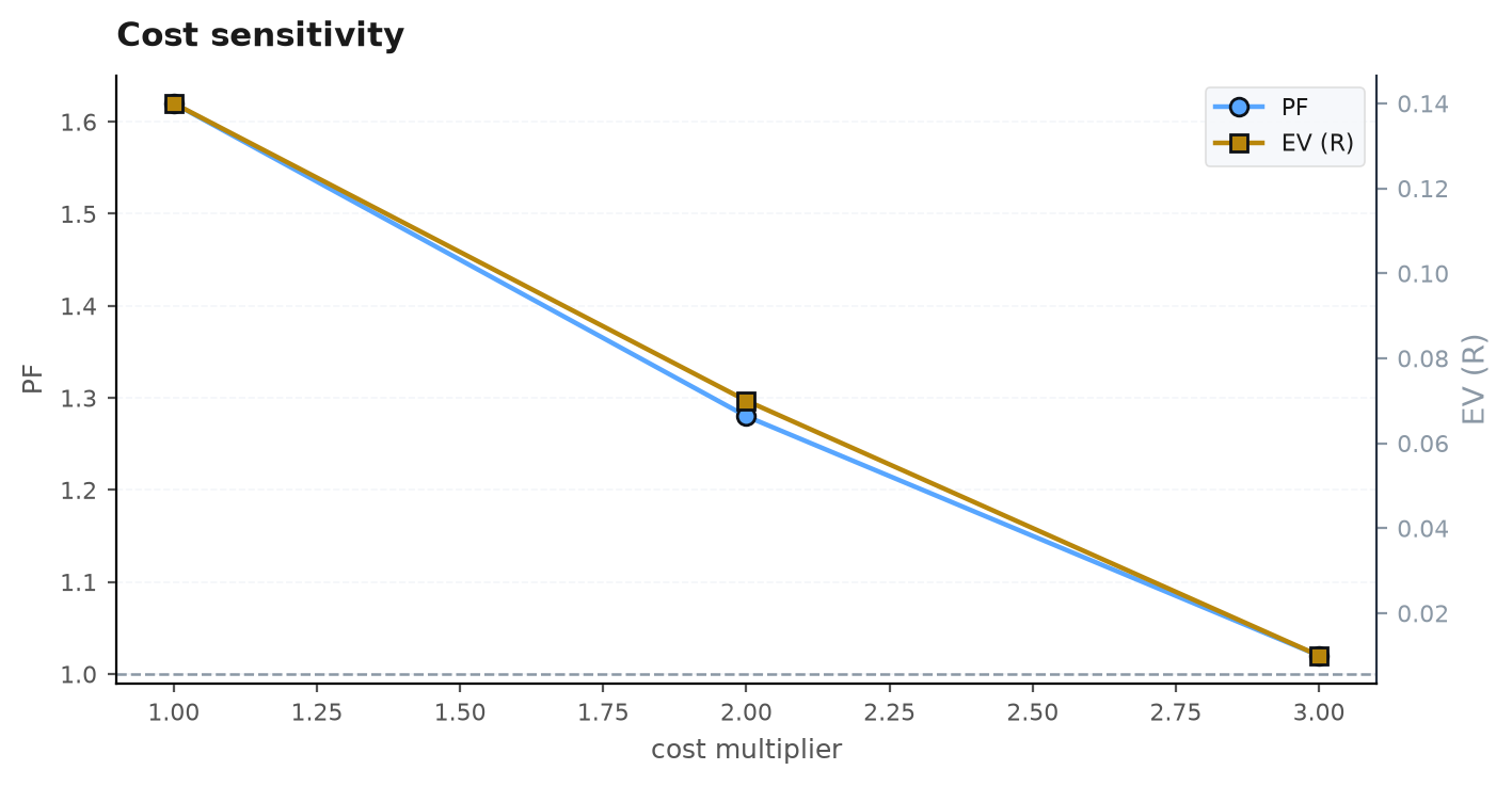
This is where strategies go to die. Every backtest looks better gross than net, and the gap is not small. There are three costs to account for.
Spread#
The gap between the best bid and best ask. You buy at the ask and sell at the bid, so you pay the spread (or half of it, each way) on everyround trip regardless of whether the trade wins. On liquid instruments it's a few basis points; on thin ones it dwarfs the edge.
Commission / fee#
An explicit charge per trade — a per-share/per-contract commission on equities and futures, a taker fee on crypto. Fixed and unavoidable, it is the second bite out of every round trip.
Swap / financing#
The cost of holding a leveraged position overnight — FX swap, CFD financing, crypto funding. Unlike spread and commission, it scales with time in the trade, so it punishes swing strategies specifically. A crossover system holding for a week pays six or seven nights of financing on top of the entry/exit costs.
edgekit rolls these into a single CostModel; the library convention is a 12 bps round-trip plus 2 bps per day held, and backtestapplies it by default. Costs are charged against the trade's risk unit, so it's natural to think of them in R. If your risk per trade is dollars and the all-in cost of a round trip is dollars, then every trade starts life down
R-multiples. If your average winner is and costs are per trade, you have handed back a tenth of your gross edge before you start. Halve the timeframe and trade twice as often, and you pay it twice as often. This is why the same signal can be a live edge on H4 and a net loser on M5.
Data quality#
The most expensive bugs in this field are not in your strategy — they are in your data, and they make bad ideas look brilliant. Three failure modes matter.
Gaps#
Missing bars. A weekend gap in FX is normal; an intraweek gap is missing data. Run one continuous backtest across a real time gap and the engine treats the jump as a single enormous bar-to-bar move — a fake trade or a fake stop-out. edgekit distinguishes the two: integrity_report counts weekend_gaps separately from intraweek_gaps.
Survivorship#
A dataset that only contains instruments that still exist today has quietly deleted every company that went to zero. A strategy tested on the survivors looks far better than it would have live, because the losers were censored after the fact. If your universe was assembled with hindsight, your backtest inherits the bias.
Look-ahead in the data#
Distinct from look-ahead in your logic: the values themselves can be contaminated. Adjusted prices that fold in a split announced later, a “final” figure that was actually a revision, a bar stamped at its close but sourced from the next period — all leak the future into the past. The defence is to look at the data before you trust it.
from edgekit import data
bars = data.load_bars("BTCUSDT_5m.csv")
rep  = data.integrity_report(bars, bar_minutes=5)
print(rep["span_days"], rep["intraweek_gaps"], rep["weekend_gaps"])
print(rep["bad_ohlc_bars"], rep["spike_bars_range_gt_20x_median"])
# look at what the data IS before any strategy touches itintegrity_report returns span, gap counts, zero-range bars, price spikes, and OHLC-invariant violations. Reading it is the cheapest insurance in the whole pipeline: a five-line check that stops you building a beautiful strategy on broken bars.Next: we set up the environment, install the library, and run a first strategy end to end in Your toolkit.