Your toolkit

Time to get your hands on the machine. This chapter sets up Python and the scientific stack, installs edgekit, and pins down the one data contract every function in the library assumes. Then we run a strategy end to end — load, resample, backtest, measure — so you have seen the whole loop turn before we slow down and take it apart.

Python and the scientific stack#

edgekit is a Python library, and its core rests on two packages you will use constantly:

numpy — fast numeric arrays. Every indicator and the backtest bar loop work on np.ndarray under the hood, because per-bar Python loops over years of data would be too slow.
pandas — labelled tables (DataFrame) indexed by time. Bars, trades, and resampling all live in pandas; the DatetimeIndexis what makes “bar i sees only bars before it” expressible.

Use a recent Python (3.10+) and, strongly recommended, a virtual environment so the install can't collide with other projects.

setup.sh

python -m venv .venv
source .venv/bin/activate      # Windows: .venv\Scripts\activate
python --version               # 3.10 or newer

Installing edgekit#

edgekit keeps a lean core (numpy + pandas only) and gates everything heavy behind extras, so you only pull in what you use. Install the extra that matches what you're doing:

Command	What you get
`pip install -e .`	Lean core: numpy + pandas. Loading, resampling, backtest, metrics, validation.
`pip install -e ".[io]"`	+ pyarrow — parquet caches and processed splits.
`pip install -e ".[viz]"`	+ matplotlib — charts and HTML tear-sheets.
`pip install -e ".[ml]"`	+ scikit-learn / xgboost / lightgbm — meta-labelling.
`pip install -e ".[all]"`	Everything (io + viz + ml + dev).

install.sh

git clone https://github.com/Atul-Ranjan12/edgekit
cd edgekit
pip install -e ".[all]"        # or ".[io]" for just parquet, or "." for the lean core

→Heavy deps are lazy

Importing edgekitdoes not import matplotlib, scikit-learn, or pyarrow. A path that needs one loads it on demand — and if it's missing you get a pointed ImportError telling you exactly which extra to install (e.g. reading a .parquet without pyarrow), not an opaque stack trace. So pip install -e . is enough to work through the CSV-based examples in this course.

Loading bars and the OHLC contract#

ek.data.load_bars reads a HistoryExporter CSV (columns time_utc,open,high,low,close,tick_volume) or a processed .parquet split. It validates the schema, sorts the index, and drops duplicate timestamps — so the frame it hands back satisfies the invariant every downstream function assumes.

load.py

import edgekit as ek
bars = ek.data.load_bars("BTCUSDT_5m.csv")
bars.head()   # DatetimeIndex(time_utc) -> open / high / low / close / tick_volume

That invariant — the OHLC contract — is worth memorising, because breaking it is the source of most silent bugs:

The index is a DatetimeIndex, tz-naive and interpreted as UTC. Session tools localise from UTC; never store a fixed local offset in the index.
It is monotone increasing and unique — sorted, no duplicate timestamps.
open, high, low, close are floats, with low ≤ open,close ≤ high on every bar.
Volume lives in tick_volume.

Keep frames in this shape and everything composes; deviate and the failure usually shows up much later as a strategy result that is subtly, expensively wrong.

Resampling to a swing timeframe#

Raw exports are often fine-grained (M1/M5). Resample up to the timeframe you actually intend to trade before doing anything else:

h4 = ek.data.resample_ohlcv(bars, "H4")   # first open, max high, min low, last close, summed vol

A first end-to-end taste#

Here is the whole loop in a dozen lines: load fine bars, resample to H4, run a strategy, and summarise the trades. We use SmaCross — a plain fast/slow moving-average crossover with an ATR stop — because it is a generic, untuned template built to exercise the engine, not an edge. That is exactly what makes it a safe first example.

first_backtest.py

import edgekit as ek

# 1. load fine bars and resample to the swing timeframe
bars = ek.data.load_bars("BTCUSDT_5m.csv")
h4   = ek.data.resample_ohlcv(bars, "H4")

# 2. run a strategy (illustrative template — not tuned, not an edge)
strat  = ek.strategy.SmaCross(fast=20, slow=100, atr_n=20, stop_mult=2.0)
trades = strat.backtest(h4, warmup=210, bars_per_day=6)   # net of the default cost model

# 3. one row per closed trade, priced in R-multiples
print(trades[["date", "dir", "r", "bars_held", "exit_reason"]].head())

# 4. summarise
st = ek.metrics.trade_stats(trades.r, dates=trades.date)
print(f"trades   : {st['n']}")
print(f"win rate : {st['win_rate']:.1%}")
print(f"expectancy (R/trade): {st['ev_r']:+.3f}")   # ev_r is E[R] per trade
print(f"profit factor       : {st['pf']:.2f}")

backtest returns the canonical trade frame — one row per closed trade with net R in r, the exit date, plus dir, bars_held, entry, exit, stop_dist, and exit_reason. trade_stats turns that R array into the universal summary: count, win rate, expectancy per trade (ev_r), profit factor, and — when you pass dates — annualised R, max drawdown, and Sharpe.

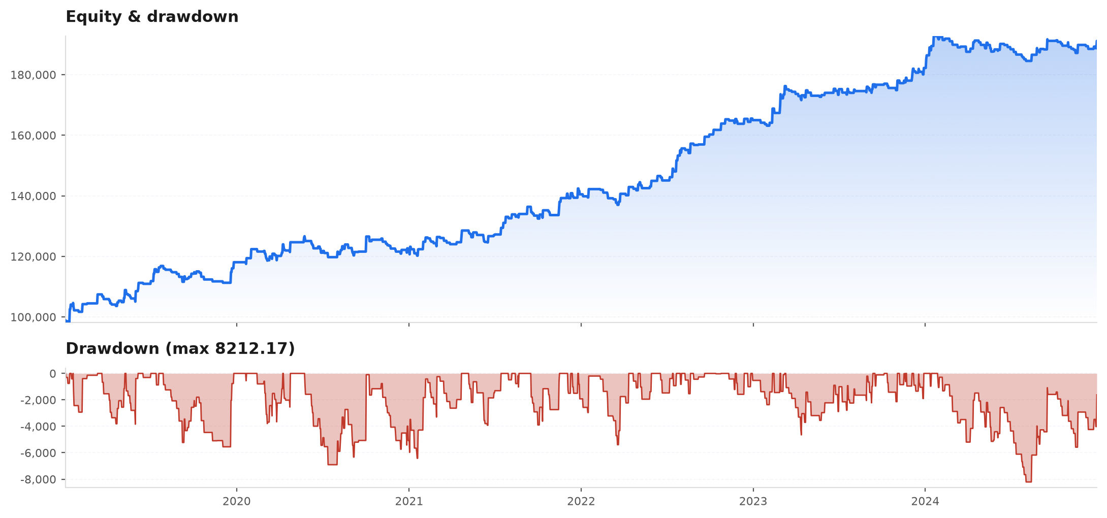
✦Scenario: reading the output like a trader

Say the print comes back trades: 184, win rate: 41.3%, expectancy: -0.021, profit factor: 0.94. Translate it at the desk: over roughly a decade of BTC H4 bars the crossover took 184 trades and won fewer than half — normal for a trend template, which wins rarely but big. The number that decides everything is the expectancy: -0.021 means theaverage trade lost about 2% of one risk unit after costs. On a $500 risk that is ~$10 bled per trade, or ~$1,840 over the whole run. Profit factor 0.94 says gross the strategy pulled in only 94 cents for every dollar it gave back. This is not a bug — it is an honest, untuned template meeting real costs and coming up short. Your job for the rest of the course is to tell this (a genuine non-edge) apart from a number that only looks like an edge.

!Expect a skeptical number

Run this and the expectancy will likely be around zero or negative once the default 12 bps + 2 bps/day cost model is applied. That is the correct, honest result for an untuned crossover — and precisely the point. A working backtest is the starting line, not the finish; the rest of the course is the machinery that tells you whether a promising-looking number is real.

If you installed the viz extra, the same trades can be drawn as an equity curve with its drawdown shaded — the first picture you will learn to read critically:

Cumulative equity curve with the drawdown from the running peak shaded beneath it — Equity curve with drawdown — the shape you'll interrogate for every strategy. A smooth-looking curve is not the same as a real edge.

What you now have#

A working environment, the library installed, the OHLC contract in hand, and one full turn of the loop behind you: load_bars → resample_ohlcv → SmaCross().backtest → trade_stats. Everything after this refines a stage of that loop.

Next, Part II opens the mathematical core with the single most consequential fact in trading — that returns multiply, they don't add — in Returns and compounding.