Monitoring a live strategy

The moment a strategy goes live, every daily P&L print poses the same question: is this drawdown noise, or death? Noise is the tuition every real edge charges; death is an edge that has decayed to zero while you keep paying to trade it. The two look identical for months, and the human default — stare at the equity curve until you feel sure — is the worst possible detector. This chapter builds the statistical machinery for the decision: sequential tests that are valid when checked every day, CUSUM alarms with calibrated false-alarm rates, the probabilistic Sharpe as a running health metric, and kill switches designed as policy, not panic.

✦Intuition — why this is hard

A strategy with true expectancy $+ 0.1$ R/day and daily noise of 1R spends roughly a third of all days losing, has losing months regularly, and will hand you a 5R drawdown somewhere in most years — while perfectly healthy. Meanwhile a strategy whose edge has died looks exactly like that, slightly worse, for a long time: the daily signal-to-noise is 0.1, so distinguishing $+ 0.1$ from $- 0.05$ takes hundreds of observations. You cannot wait for certainty — the dead strategy burns money the whole time — and you cannot react to every drawdown, or you will kill healthy strategies at exactly their cheapest moments. Monitoring is the discipline of pre-committing to the best achievable trade-off between those two errors.

Why you can’t just re-run the t-test every day#

The tempting procedure — each evening, t-test the live mean against zero, act when $p < 0.05$ — is statistically broken. The 5% false-alarm guarantee holds for one look at the data. Look every day and you take hundreds of shots at a 5% target; by the law of the iterated logarithm a random walk is guaranteed to cross any fixed significance boundary eventually, so the daily-peek procedure kills every healthy strategy with probability one — it is the multiple-testing problem smeared across time. The fix is a genuinely sequentialtest: a statistic designed to be monitored continuously, whose false-alarm rate is controlled over the whole monitoring horizon. That theory exists — Wald’s SPRT and its process-control descendant, the CUSUM.

CUSUM: the sequential change detector#

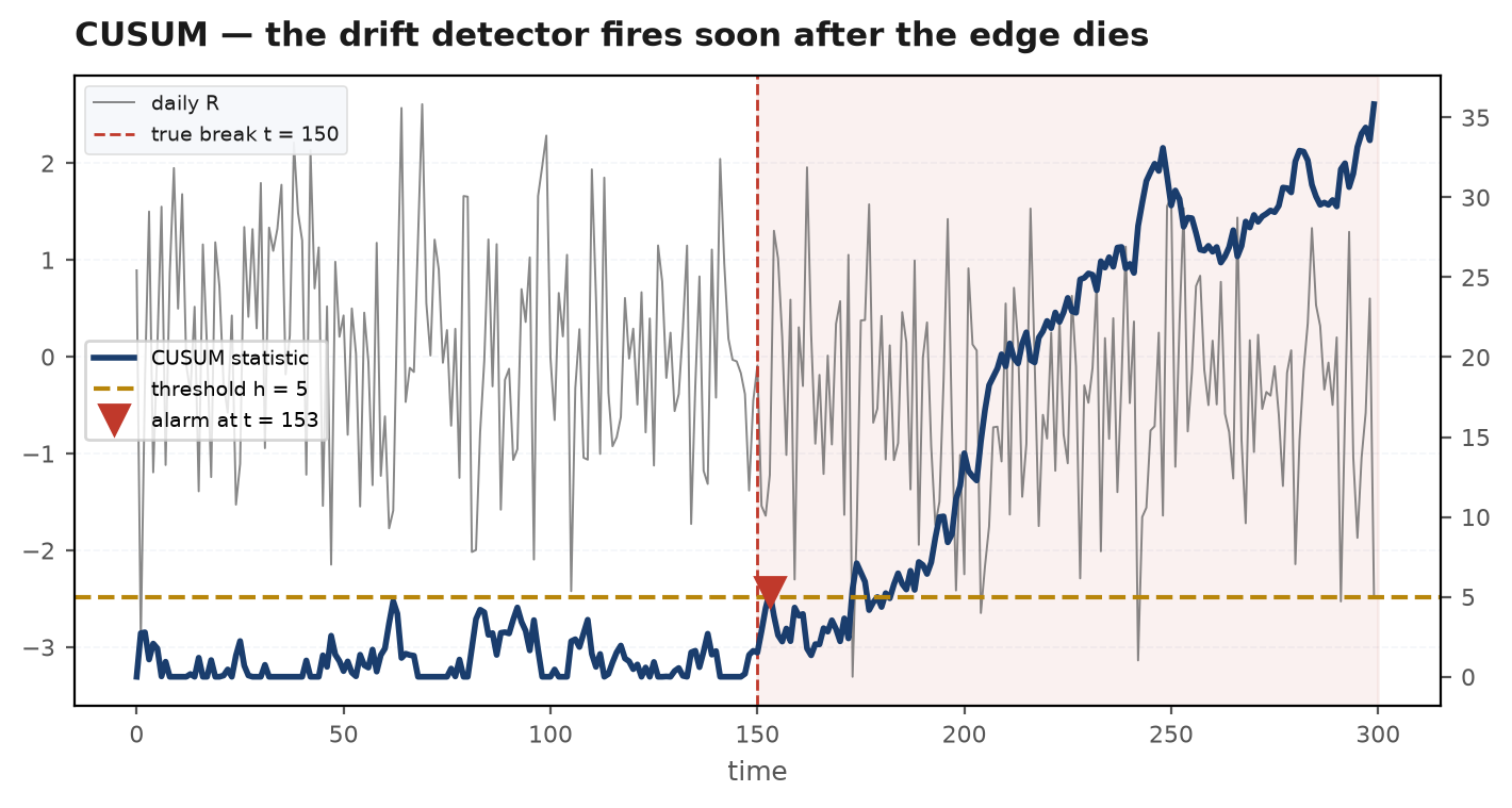
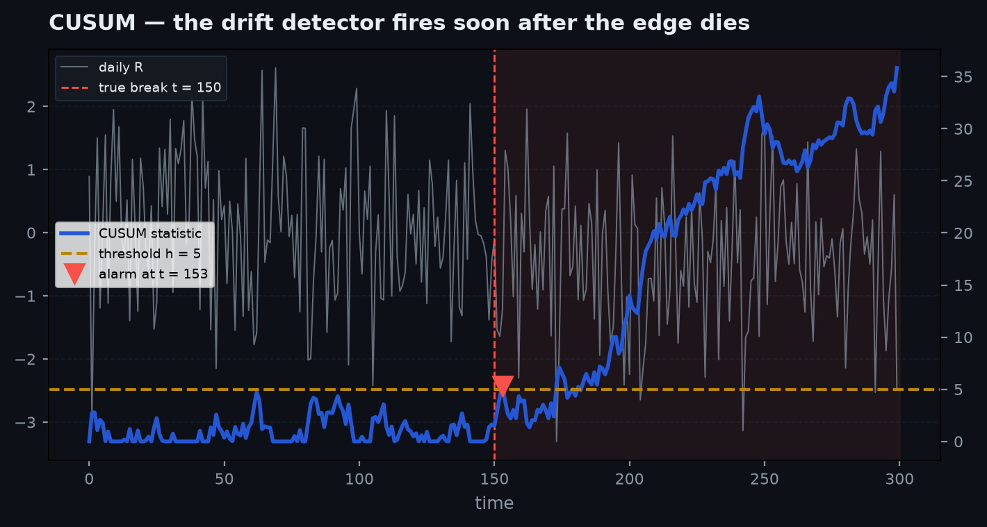
Standardise each day’s return against the backtest’s claim: $z_{t} = (r_{t} - μ_{bt}) / σ_{bt}$ . The one-sided (lower) CUSUM accumulates evidence of deterioration:

S_{t} = max (0, S_{t - 1} + (- z_{t}) - k), alarm when S_{t} > h .

Good days push $S_{t}$ down (never below zero — the reset is the point); bad days push it up by more than the allowance $k$ . A healthy strategy’s statistic keeps draining back to zero; a dead one’s climbs at a steady rate until it crosses $h$ .

✦Derivation — SPRT intuition, and calibrating k and h

Wald’s sequential probability ratio test tracks the log-likelihood ratio between two hypotheses. For Gaussian returns, testing “mean shifted down by $δ$ ” against “mean as claimed,” each day’s log-likelihood increment is proportional to $- z_{t} - δ /2$ . The CUSUM is exactly this running SPRT, restarted at zero whenever the evidence favours health (Page, 1954) — which is why it is optimal (Moustakides) for detecting a shift of size $δ$ as fast as possible at a given false-alarm rate. The recipe:

Set $k = δ /2$ — half the shift you care to detect, in sigma units. Detecting a fall from $+ 0.1$ R to $- 0.05$ R with 1R daily noise means $δ = 0.15$ , so $k = 0.075$ .
Set $h$ from the ARL — the average run length to a false alarm while healthy. Raising $h$ buys a longer healthy ARL at the price of slower detection: once dead, the statistic drifts up at $δ - k = δ /2$ per day, so detection delay $\approx h / (δ - k)$ . Choose the false alarm you can live with (one per several years), read off $h$ , and accept the delay that implies. There is no setting with fast detection and no false alarms — only the frontier.

A live equity curve above and its CUSUM statistic below: the statistic rises and drains during a transient drawdown, then climbs steadily through the threshold h after the true edge dies, with the alarm marked — CUSUM on a live R stream. A transient (lucky-noise) drawdown lifts the statistic, then recoveries drain it back toward zero. After the true edge dies, there are no recoveries to drain it — the statistic grinds upward at ~delta/2 per day and crosses h. The alarm fires on accumulated evidence, not on a scary week.

→Monitor the upside too

The same machinery run on

+ z_{t}

detects a strategy performing too well — which sounds like a nice problem until you remember what it usually means: a risk mis-scaling, a leaked position doubling, or a regime handing you beta you did not sign up for. Symmetric surprise deserves symmetric investigation; the upper CUSUM is the cheapest bug detector you will ever run.

The probabilistic Sharpe as a monitor#

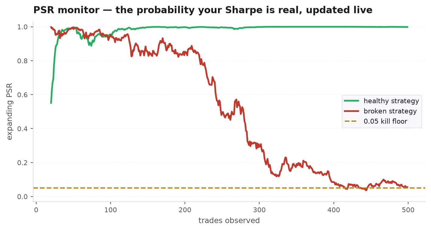
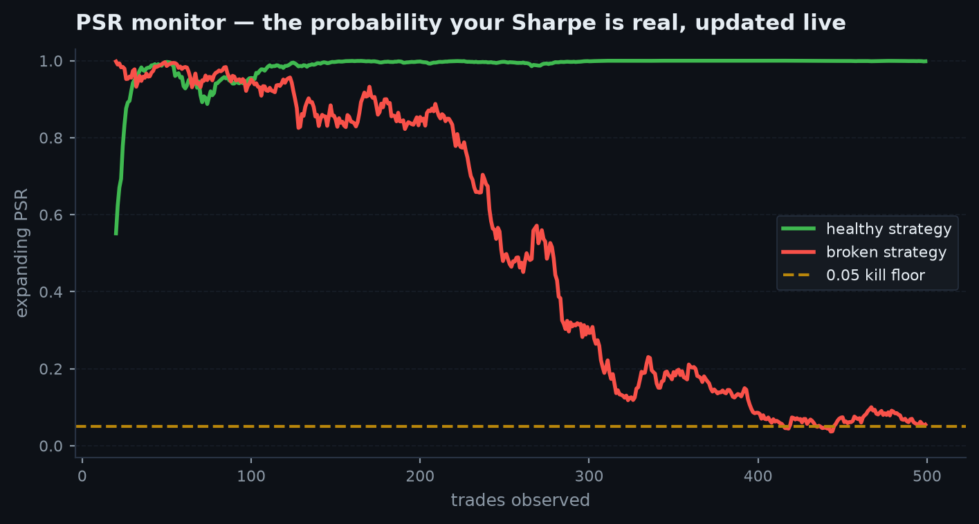
The CUSUM answers “has something changed?” The probabilistic Sharpe ratio answers the complementary question: given everything live so far, what is the probability the true Sharpe exceeds a benchmark? PSR takes the observed Sharpe and its sampling error — inflated by the skew and fat tails your return distribution actually has — and returns $Pr (SR > SR_{bench})$ . Tracked on an expanding window (ek.monitor.psr_monitor), it is the honest confidence gauge: early on it hovers near 0.5 (you know nothing), and it should grind upward as a real edge accumulates evidence. A PSR that stalls below 0.5 for months is a strategy failing to prove it is better than nothing — softer evidence than a CUSUM alarm, and earlier.

Expanding-window probabilistic Sharpe ratio through time for a healthy strategy grinding up toward one, and a dying strategy stalling and sliding below one half — Expanding PSR as a health gauge. The healthy strategy's probability of a positive true Sharpe grinds upward with evidence; the dying one stalls near a coin-flip and slides. Crossing a pre-set floor is a kill-switch input, not a suggestion.

Backtest-vs-live reconciliation#

Alarms detect that live returns are worse than claimed; reconciliation asks where the gap comes from. Two complementary audits, run monthly:

Distribution test. ek.monitor.reconcileruns a Welch t-test between the backtest’s daily R distribution and the live one. A significant mean gap with similar shapes points at costs; a changed shape (fatter left tail, missing right tail) points at fills, regime, or a bug.
Slippage audit. Per trade, compare modelled cost against realised implementation shortfall from the execution chapter. If live slippage runs 2x the model, the backtest’s edge was measured with the wrong ruler — fix the cost model before blaming the signal.

This is the live continuation of the paper-trading reconciliation in from backtest to live: divergence is a bug report first and a verdict on the edge second. Keep the expectation honest, though — with 60 live days against 1,000 backtest days, the Welch test only has power to detect gaps of ~0.35R/day or more; a “non-significant” result is absence of evidence, not evidence the distributions match. The reconciliation earns its keep on the direction and structure of the gap long before the p-value clears.

Kill switches: policy, not panic#

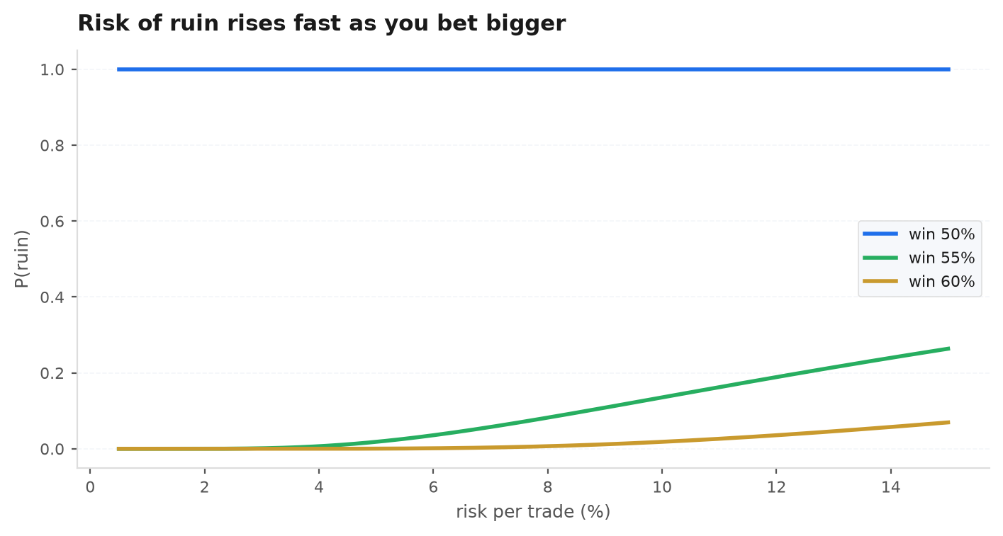
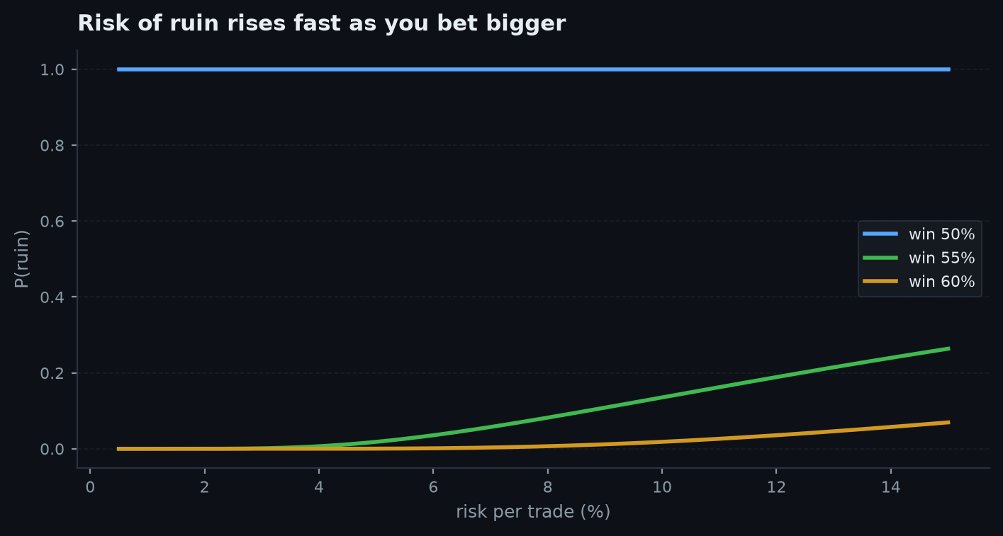
The final layer is the pre-committed decision rule — written down before going live, when you are calm, so that the worst week executes a checklist instead of an argument. ek.monitor.KillSwitch bundles the triggers: a maximum drawdown, a PSR floor, and CUSUM parameters; check(live_r) returns a verdict and its reasons. The drawdown line belongs to risk management (ruin protection — see also the hard daily-loss rails in prop-firm capital); the PSR and CUSUM lines belong to inference (edge-death detection). Both matter, and they fire on different timescales.

Probability of ruin as a function of risk per trade, rising steeply past a threshold — From the risk chapter: ruin probability vs risk. The kill switch's drawdown line is the ruin guard; the CUSUM and PSR lines guard against the slower death of paying costs to trade an edge that no longer exists.

Worked scenario — alarm timing when the edge dies#

✦Scenario: +0.1R/day backtested; live truth drops to −0.05R/day

You deploy a strategy whose gauntlet-surviving backtest claims $μ = + 0.1$ R/day, $σ = 1$ R. You care about the shift to $- 0.05$ R/day — a dead edge still paying costs — so $δ = 0.15$ , $k = 0.075$ , and you pick $h = 6$ for a healthy ARL in the thousands of days (a false alarm perhaps once a decade). Two futures:

The edge is dead from day one. The statistic climbs at $δ - k = 0.075$ /day on average and crosses $h = 6$ after roughly $6/0.075 \approx 80$ trading days — about four months. Painful, but compare the alternative: a fixed-sample t-test would need $n \approx (2.8/0.15)^{2} \approx 350$ days for comparable error rates, and the daily-peek version would have destroyed its own error control entirely.
Healthy, but a lucky-noise drawdown. The strategy hits a 5R drawdown over six weeks — frightening, but its bad days are interleaved with recoveries, and each good day drains $S_{t}$ . The statistic peaks around 3-4 and subsides without crossing 6. The CUSUM held your hand through exactly the episode where an unaided human pulls the plug at the bottom.

The 80-day delay is not a flaw — it is the price, set by signal-to-noise, of not being fooled by six-week drawdowns. The only dials that shorten it honestly are a bigger $δ$ you are willing to tolerate, or more independent bets per day.

monitor.py

import edgekit as ek

# live_r: Series of live daily R; bt_r: the backtest's daily R stream
# 1. sequential change detection (standardised internally against the stream's claim)
cu = ek.monitor.cusum(live_r, k=0.075, h=6.0)
print(f"S_t = {cu['stat'].iloc[-1]:.2f}, alarms at: {cu['alarms']}")

# 2. expanding probabilistic Sharpe — the confidence gauge
psr = ek.monitor.psr_monitor(live_r, sr_benchmark=0.0, min_obs=20)

# 3. monthly reconciliation: is live drawn from the backtest's distribution?
rec = ek.monitor.reconcile(bt_r, live_r)
print(f"mean gap {rec['mean_gap']:+.3f}R/day (t={rec['t_stat']:.2f}, p={rec['p_value']:.3f})")

# 4. the pre-committed policy, checked daily
ks = ek.monitor.KillSwitch(max_dd=0.10, psr_floor=0.05, cusum_h=6.0, cusum_k=0.075)
verdict = ks.check(live_r)
if verdict["kill"]:
    print("FLATTEN:", ", ".join(verdict["reasons"]))

Monitor	Detects	Timescale	On trigger
Daily-loss / max-DD rail	Ruin risk, fat-tail day	Immediate	Flatten now, review later
CUSUM alarm	Sustained mean shift (edge death)	Weeks-months	Halve size, start review
PSR floor	Failure to accumulate evidence	Months	Probation: no size increases
Reconciliation gap	Cost model / fill / bug divergence	Monthly audit	Fix pipeline before judging edge

!Write the rules before you need them

Every threshold above must be chosen before the first live trade, while you have no position and no P&L to rationalise. A kill switch designed mid-drawdown is not a policy — it is panic with parameters. And the symmetric failure is real too: overriding a fired alarm (“it’s about to turn”) converts a bounded loss into an unbounded one. The rule you will not follow is worse than no rule, because it spends your discipline budget pretending.

Next: monitoring is the last feedback loop in the deployment pipeline — revisit from backtest to live to see where these monitors slot into the full haircut-paper-deploy sequence, then take the whole course end-to-end in the capstone.