Market microstructure

A backtest fills you at the close, instantly, in any size. The real market is a queue of resting orders you have to cross, and every crossing costs money you did not model. Microstructure is the study of how that queue works — how prices actually form, why there is a spread between what you can buy and sell at, and where the frictions in your P&L come from. This chapter builds the limit order book from the bottom up and decomposes the spread into its economic parts, then ties each back to the cost you charge in a backtest with ek.costs.CostModel.

✦Why a trader cares

Your backtest bought 5,000 shares of a stock at exactly $50.00, the closing print. In the real market there was no one offering 5,000 shares at $50.00 — there were 800 at $50.01, 1,200 at $50.02, and so on up the ladder. You paid a blendedprice above the quote, and that difference, times every trade you will ever make, is a tax your P&L never saw coming. This chapter opens up the machinery — the order book, the spread, who pays whom — so that when you charge a cost in ek.costs you know exactly what real thing that number stands for.

The limit order book#

Modern electronic markets are continuous double auctions. Every resting order lives in the limit order book (LOB): a price-sorted ladder of bids (buyers, below) and asks/offers (sellers, above). Each level shows a price and the total quantity waiting there — the depth. The two prices that matter most sit at the inside of the book:

spread = P_{ask} - P_{bid}, mid = \frac{P _{bid} + P _{ask}}{2}

The best bid is the highest price a buyer will pay; the best ask the lowest a seller will accept. The midis the usual reference “price” — but you can never trade at the mid with a market order: you buy at the ask and sell at the bid. That gap is the first cost of doing business.

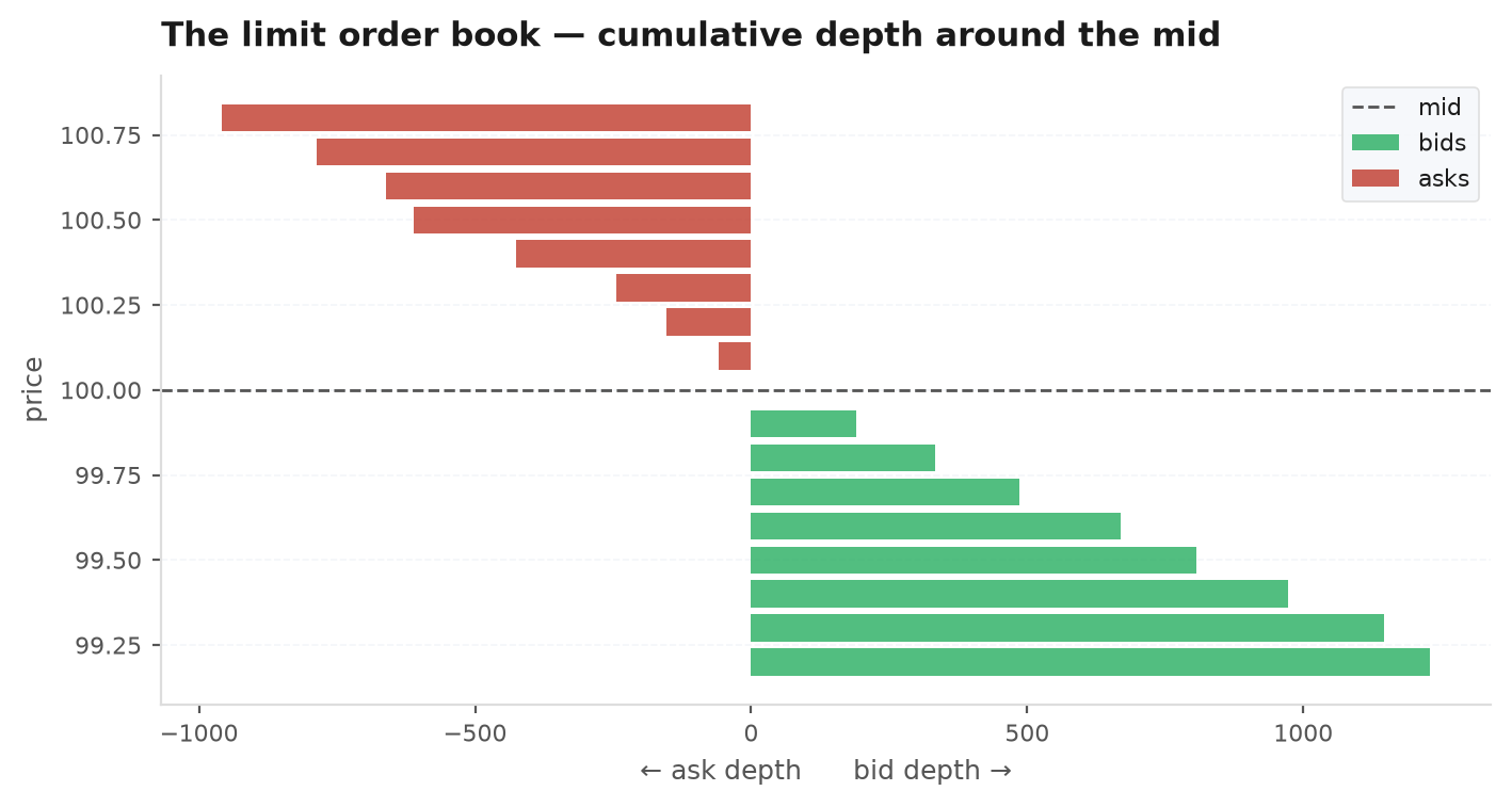
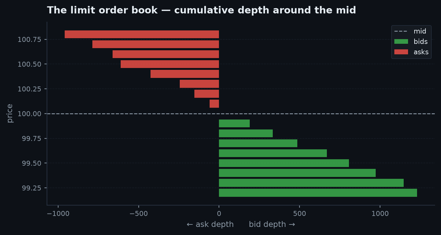
A limit order book drawn as horizontal bars: green bid depth stacked below the mid price, red ask depth above, with the bid-ask spread marked at the inside — A snapshot of the book. Bid depth (below) and ask depth (above) are quantities resting at each price. The inside spread separates the best bid and best ask; the mid sits between them. A market buy walks up the ask ladder, consuming depth.

A market order that is larger than the depth at the inside walks the book: it fills the first level, then the next, then the next, at progressively worse prices. The average fill is therefore worse than the inside quote — the origin of market impact, covered in the next chapter. A backtest that assumes you always transact at the mid silently ignores both the spread and this walk.

✦Scenario: a book snapshot and a market buy that walks it

Here is a snapshot of a $50 stock on a 1-cent tick. Asks (sellers) above, bids (buyers) below:
ask 50.04 × 3000 | 50.03 × 2000 | 50.02 × 1500 | 50.01 × 800
bid 50.00 × 1000 | 49.99 × 1800 | 49.98 × 2500
The best bid is $50.00, the best ask $50.01, so the quoted spread is exactly one tick ($0.01) and the mid is $50.005. Now send a market buy for 5,000 shares. There are only 800 at the inside, so you walk up: 800 @ 50.01, 1,500 @ 50.02, 2,000 @ 50.03, and the last 700 @ 50.04. Total cost

= $250, 126

, so your average fill is $50.0252 — about 2 cents (≈4 bps) above the mid, even though the screen showed a 1-cent spread. A backtest filling all 5,000 at $50.005 just handed you $101 of free money that the book never offered.

Market orders vs limit orders#

Every trade is one of two roles:

Market order (liquidity taker): execute immediately against the resting book. You are guaranteed a fill but you pay the spread and any impact — you cross from mid to ask (buying) or mid to bid (selling). Certainty of execution, uncertain price.

Limit order (liquidity maker): post a resting order at your chosen price and wait. If it fills, you earn the spread instead of paying it (and often a maker rebate). But there is no guarantee it fills at all — and worse, it tends to fill precisely when you did not want it to (adverse selection, below). Certain price, uncertain execution.

→The maker-taker asymmetry is the whole cost story

A taker's cost is a maker's income. The spread you pay crossing the book is (roughly) the compensation the resting side earns for providing immediacy and bearing the risks that follow. Understanding why that compensation exists is understanding the spread.

Tick size and price formation#

Prices are not continuous — they move on a discrete grid, the tick size, the minimum increment between quotable prices. Tick size sets a floor on the spread: it can never be tighter than one tick. In a liquid, large-tick instrument the spread is often pinned at exactly one tick and the real competition is for queue priority at that price, not for price itself. In a small-tick instrument the spread floats and depth thins out.

Price formation is the process by which this book turns order flow into a consensus price. Each arriving market order and each cancellation nudges the inside quotes; the mid drifts as buyers and sellers reveal their willingness to pay. Price is not handed down — it is discovered, one order at a time, and the spread is the friction in that discovery.

The three components of the spread#

Why is there a spread at all, and what sets its width? The market-making literature decomposes it into three economic parts a liquidity provider must be paid for:

spread = order processing c_{proc} + inventory c_{inv} + adverse selection c_{adv}

Order-processing cost#

The fixed operational cost of making a market — exchange fees, clearing, technology, and a minimum profit for the service of standing ready to trade. This is the floor and the smallest, most stable component.

Inventory cost#

A market maker who buys from a seller now holds inventory they did not want and bears the risk that the price moves against it before they can offload it. They widen the quote to be compensated for this warehousing risk, and they skew the quote to nudge their inventory back toward flat. The more volatile the asset, the larger this component — which is why spreads widen precisely when volatility spikes.

Adverse selection#

The deepest component, and the reason posting limit orders is dangerous. Some of the flow hitting the market maker is informed— it trades because it knows something about where the price is going. When an informed buyer lifts the maker's offer, the price is about to rise, so the maker just sold too cheap. The maker cannot tell informed flow from noise ex ante, so they widen the spread on everyone to recover, on average, what they lose to the informed. Adverse selection is the market maker's payment for trading against people who know more than they do.

!Adverse selection is why your limit orders fill at the wrong time

A resting buy limit fills when someone sells to you — disproportionately, when they have a reason to sell, i.e. when the price is about to drop. “My limit orders always fill right before the market moves against me” is not bad luck; it is the structural signature of adverse selection. It is also why the spread cannot be modelled away: it is priced-in information asymmetry.

✦Scenario: watch the spread widen when the three costs rise

On a calm morning a liquid ETF quotes 100.00 / 100.01 — a 1-cent spread that is almost pure order-processing cost, because volatility is low (small inventory risk) and flow is mostly uninformed retail (little adverse selection). Then a Fed headline hits. Volatility triples, so a maker who buys now faces a much larger chance the price runs against their inventory before they can offload it — inventory cost jumps. And the flow turns sharp: the orders arriving are increasingly informed traders repricing the news, so adverse selectionjumps too. The maker's only defence is to widen: the quote gaps to 99.96 / 100.04, an 8-cent spread. Nothing about the ETF changed — the cost of providing liquidity did. That is why your slippage is always worst in exactly the fast market where you most want to trade.

Quoted vs effective spread#

The quoted spread is what you see: $P_{ask} - P_{bid}$ . The effective spread is what you actually paid, measured against the mid at the moment of your trade — and for anything larger than the inside depth it is wider, because you walked the book:

S_{eff} = 2 P_{fill} - P_{mid}

The factor of 2 makes it comparable to a full round-trip quoted spread (one side of the crossing, doubled). The gap between effective and quoted spread is your impact: the effective spread is the honest, trade-weighted cost, and it is the number a realistic backtest must charge — not the flattering inside quote.

✦Scenario: quoted vs effective on the same 5,000-share buy

Take the book-walk above. The quoted spread was $0.01. But you filled at an average of $50.0252 against a mid of $50.005, so your effective spread is

S_{eff} = 2 ∣50.0252 - 50.005∣ = $0.040

— four times the quoted spread. That factor of 4 is the size penalty: the quote describes the first 800 shares, the effective spread describes all 5,000. As a fraction of price it is

0.040/50 \approx 8 bps

round-trip-equivalent — and that 8 bps, not the flattering 2 bps quoted spread, is what belongs in your cost model for an order this size.

Tying it back to ek.costs#

You will not simulate the full order book in a strategy backtest — you compress all of the above into a single cost charged per round trip. That is exactly what ek.costs.CostModel does. Its spread_rt parameter is the round-trip spread as a fraction of price: it stands in for the quoted spread plus the typical impact of your size — i.e. an estimate of the effective spread you will pay crossing the book twice. Its swap_day is the financing/carry per day held.

costs.py

import edgekit as ek

# 12 bps round-trip spread, 2 bps/day financing (a crypto/CFD convention)
cm = ek.costs.CostModel(spread_rt=0.0012, swap_day=0.0002)

# cost of one round trip, expressed in R (dollar cost / the stop-distance risk unit)
r_cost = cm.r_cost(entry_price=100.0, risk_per_unit=2.0, days=3)
print(round(r_cost, 4))          # subtract this from every trade's gross R

✦At the desk: from the book snapshot to spread_rt

The effective spread you measured on the 5,000-share buy was ≈8 bps one way. You cross twice per round trip, so a realistic spread_rt for that instrument and size is on the order of

0.0016

(16 bps), not the 12-bps placeholder. If your stop distance is $2 on a $50 entry, the round-trip dollar cost is

0.0016 \times 50 = $0.08

, which is

0.08/2 = 0.04 R

gone before the trade even works. A signal with 0.15R of gross expectancy just lost a quarter of its edge to the book — and that is before the cost stress in the next chapter doubles it.

The microstructure lesson is why this subtraction is not optional. The spread is not noise you can average away — it is a structural transfer from taker to maker on every trade, set by inventory risk and adverse selection, and it scales with how often you trade and how hard you cross. A high-frequency signal pays the effective spread hundreds of times; a slow one pays it rarely. Which cost dominates, and whether a gross edge survives it at all, is the subject of the next chapter.

✦Estimate spread_rt from the real book, not a default

The 0.0012 default is a placeholder. Pull the actual quoted spread and typical depth for your instrument and size, widen it toward the effective spread for the size you trade, and — as always — re-run at 2x and 3x that estimate to see whether the edge is real or a rounding artefact.

Next: Execution & transaction costs — slippage, the square-root impact law, execution algos, and the transaction-cost analysis that decides whether a signal is tradeable.