Execution & transaction costs

A signal is only half a strategy. The other half is getting the trade done at a price close enough to the one your backtest assumed that the edge survives. Most researched edges are real on paper and dead in production for one reason: execution costs. This chapter quantifies where those costs come from — slippage and market impact, temporary and permanent — states the square-root impact law, walks through the execution algos that manage it, defines implementation shortfall as the honest scorecard, and shows how transaction-cost analysis and capacity limits decide whether a signal is worth trading at all.

✦Why a trader cares

You have a signal that makes 12 bps per trade on paper. You scale it up, and at $2m per order it still works. At $20m per order it is flat. At $50m it loses money — same signal, same market, same code. Nothing broke except that your orders got big enough to move the price against themselves. This chapter is the arithmetic of that collapse: how much a trade costs to execute, why cost grows with size, and how to tell — before you commit capital — whether an edge is a real business or a paper mirage that dies on contact with the book.

Why execution matters#

The trap is the difference between gross and net edge. A signal with a healthy gross profit factor can have a negative net one the moment costs are subtracted — and the faster it trades, the more times it pays. From the metrics chapter, an edge is judged on expectancy in R; costs are subtracted from every trade before that expectancy is computed:

E [R_{net}] = E [R_{gross}] - c_{R}, c_{R} = \frac{cost per round trip}{risk per unit}

When $c_{R}$ approaches gross expectancy, the edge vanishes. This is not a haircut you apply at the end — it is a survival test. A great signal dies on costs quietly: the equity curve just tilts a few basis points per trade until it points down.

Slippage and market impact#

Slippage is the gap between the price you expected and the price you got. Part of it is the spread from the last chapter; the rest is market impact — the fact that your own order moves the price against you as it consumes liquidity. Impact splits into two kinds:

Temporary impact is the concession you pay for demanding immediacy: you walk the book, depth refills after you are done, and the price snaps back. It is a cost of how you traded and it decays.

Permanent impactis the information your trade reveals: the market infers that a large buyer knows something, and the price stays elevated. It is a lasting shift in the mid that does not come back — the adverse-selection cost from the previous chapter, seen from the taker's side.

The square-root law#

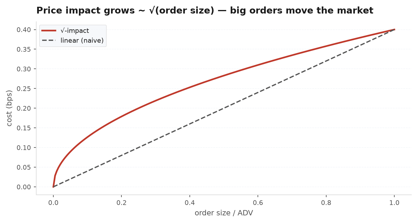
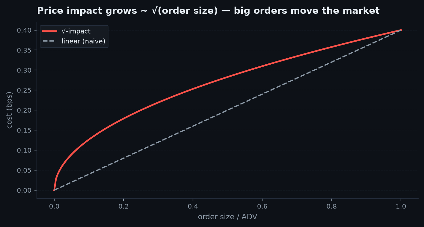
The central empirical regularity of impact: the price concession from trading a quantity $Q$ against a daily volume $V$ grows not linearly but as the square root of participation:

impact \propto σ \frac{Q}{V}

where $σ$ is the asset's volatility and $Q / V$ the fraction of daily volume you represent. Two consequences drive everything downstream. First, impact is concave: doubling your size less-than-doubles your cost, so there is a real benefit to trading larger — up to a point. Second, and more important, cost per share rises with size ( $Q / V / Q \propto 1/ Q$ falls, but total impact still climbs), and the $Q$ term is what eventually caps a strategy's capacity.

Market impact plotted against order size as a fraction of daily volume, a concave square-root curve rising steeply for small sizes then flattening — The square-root impact law. Cost rises with participation but concavely — the first slice of size is cheap per share, later slices climb. Trading faster (higher Q/V per unit time) pushes you up this curve.

✦Scenario: impact on an order that is 10% of a day's volume

A $50 stock trades

V = 10

million shares a day with daily volatility

σ = 2%

. You need to buy

Q = 1

million shares — that is

Q / V = 10%

of the day's volume, a genuinely large order. With a calibrated coefficient

c \approx 0.5

, the square-root law estimates

impact \approx c σ Q / V = 0.5 \times 0.02 \times 0.10 \approx 0.0032

— about 32 bps, or 16 cents a share, roughly $160k on the $50m notional. Now feel the concavity: had you needed only 100k shares (

Q / V = 1%

), impact would be

0.5 \times 0.02 \times 0.01 = 10 bps

— so a 10× larger order costs only ~3× the impact (

10 \approx 3.2

), the hallmark of the square root. The flip side is timing: to actually get the 32-bps number you must trade the million shares slowly across the day so your instantaneous participation stays low — and while you drip it out, the price can drift away from you. Impact versus timing risk is the entire job of an execution algo.

Execution algorithms#

The whole job of an execution algo is to manage the trade-off the square-root law creates: trade too fast and you pay impact; trade too slow and you carry timing risk — the price may drift away before you finish. Three canonical schedules:

TWAP (time-weighted average price): slice the order into equal pieces spaced evenly over a fixed window. Simple, predictable, ignores volume — good when you want a steady, low-footprint schedule and do not trust volume forecasts.

VWAP (volume-weighted average price): slice in proportion to expected volume, trading more when the market is busy and less when it is thin. The benchmark most institutions are measured against, because participating in proportion to volume minimises footprint for a given size.

POV (percentage of volume): trade a fixed fraction of whatever volume actually prints in real time — say 10% of every trade — so your participation is capped no matter how the day develops. Adapts to realised liquidity at the cost of an uncertain completion time.

✦Scenario: three ways to work the million shares

Same 1m-share buy on the $50 stock. TWAP over 6.5 hours slices it into, say, 78 equal clips of ~12,800 shares every 5 minutes — steady and predictable, but it buys just as hard into the thin lunch lull as into the busy open, leaving a visible footprint when volume dries up. VWAP instead front- and back-loads to match the U-shaped intraday volume curve — heavier at the 9:30 open and 4:00 close, lighter midday — so it keeps participation near a constant ~10% of actual volume and minimises footprint. POV at 10%stops asking the clock and simply takes 10% of whatever prints: if a block trade doubles the day's volume you buy more; if the tape goes quiet you buy less and may not finish by the close. None is free — TWAP ignores liquidity, VWAP trusts a volume forecast, POV surrenders your completion time.

→Every algo is a point on the impact-vs-timing frontier

There is no free schedule. Front-loading cuts timing risk but raises impact; stretching out cuts impact but raises timing risk. The optimal trajectory (Almgren-Chriss and its descendants) trades off expected impact against the variance of the fill — the same risk/return logic as the rest of this course, applied to a single order.

Implementation shortfall#

The honest scorecard for execution is implementation shortfall (IS): the difference between the price at the moment you decided to trade (the decision or arrival price) and the average price you actually filled at, plus the opportunity cost of anything you failed to execute:

IS = execution cost Q (P ˉ_{fill} - P_{decision}) + opportunity cost (Q - Q_{filled}) (P_{end} - P_{decision})

IS captures what a backtest hides. Your backtest fills at $P_{decision}$ (or worse, the close); reality fills at $P ˉ_{fill}$ after spread, impact, and delay. The shortfall is the leakage between simulated and live P&L — and it is precisely the quantity your cost model is trying to estimate in advance.

✦Scenario: scoring the fill with implementation shortfall

You decide to buy the million shares when the stock is at

P_{decision} = $50.00

. Working it with VWAP, you fill 950,000 shares at an average of $50.08, but the tape runs and you never get the last 50,000 before the stock closes at $50.20. Score it:
• Execution cost =

950, 000 \times (50.08 - 50.00) = $76, 000

— what you paid above your decision price on the shares you got.
• Opportunity cost =

50, 000 \times (50.20 - 50.00) = $10, 000

— the profit you forfeited on the shares you failed to buy while the price moved away.
Total IS =

$86, 000

, or

86, 000/ (1 0^{6} \times 50) \approx 17 bps

of the intended notional. Your backtest, filling all 1m shares instantly at $50.00, recorded zero of this. IS is the honest gap between that fantasy and the trade you actually did.

Transaction-cost analysis#

TCA is the post-trade discipline of measuring realised execution cost — decomposing each fill into spread, temporary impact, permanent impact, and timing — and feeding it back into both the cost model and the choice of execution algo. In research you run TCA forward: you assume a cost, and then you stress it. edgekit's harness does exactly this — re-run the strategy at escalating multiples of your baseline cost and watch what happens to the metrics:

cost_stress.py

import edgekit as ek

def run(cost: ek.costs.CostModel) -> dict:
    r = backtest_returns_in_R(cost)          # your strategy, charged this cost
    return ek.metrics.trade_stats(r)

grid = ek.validation.cost_stress(
    run,
    base=ek.costs.CostModel(spread_rt=0.0012, swap_day=0.0002),
    mults=(1.0, 2.0, 3.0),
)
for m, stats in grid.items():
    print(f"{m}x cost -> PF {stats['pf']:.2f}, EV {stats['ev_r']:.3f}R")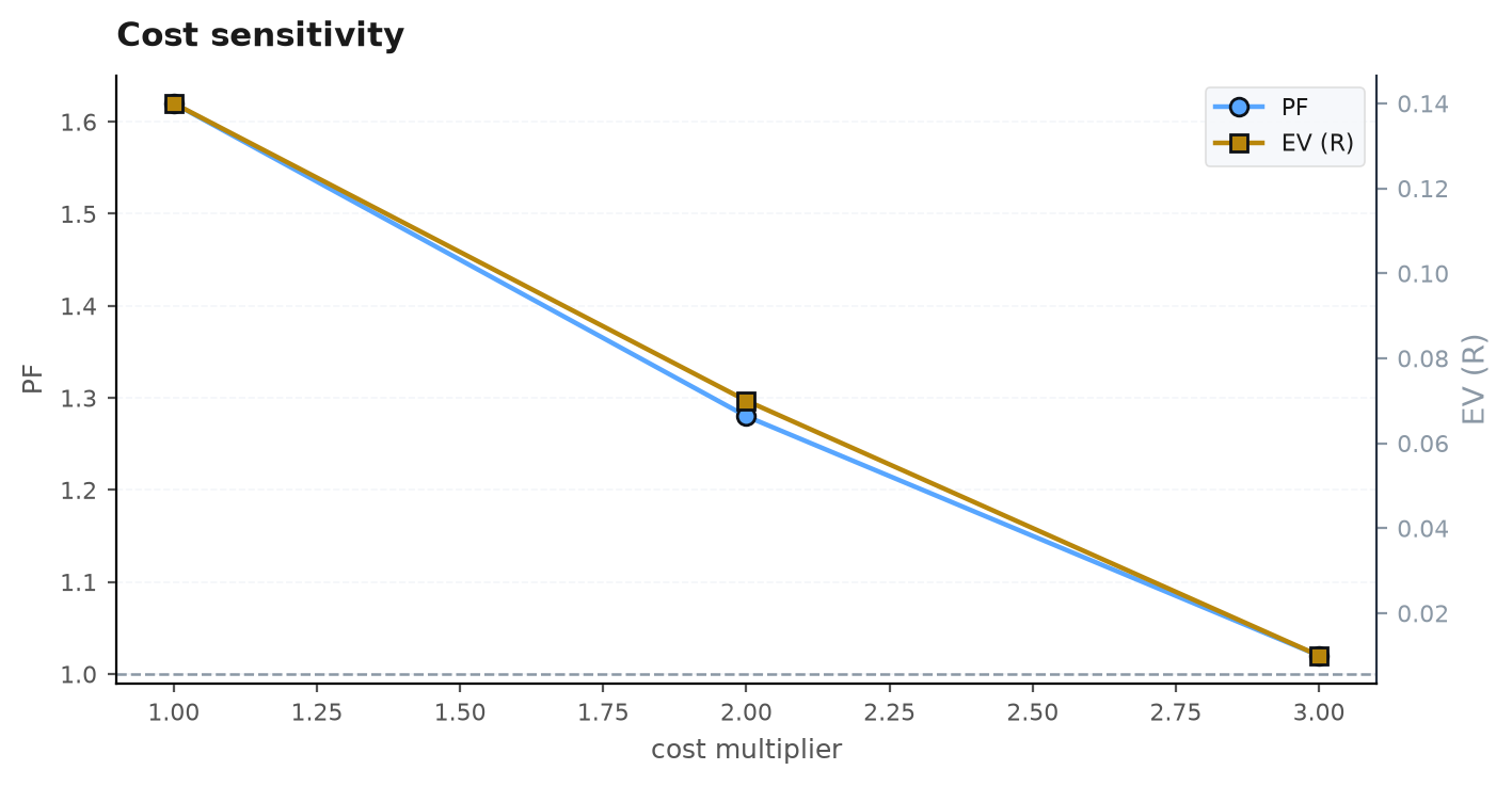

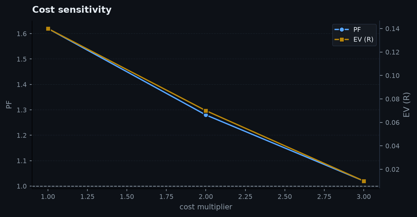
Profit factor plotted against a cost multiplier, showing a robust edge degrading gracefully while a fragile one collapses below 1 — Cost sensitivity. A real edge (upper line) degrades gracefully as cost rises; a fragile one (lower) crosses PF = 1 by 2-3x and was never tradeable. The survivor rule: PF must stay above 1 at 2x and 3x.

The survivor rule of thumb is blunt: profit factor must stay above 1 at 2x and 3x your baseline cost. A genuine edge has margin; a curve-fit one is a knife-edge that the first realistic cost estimate tips over. This is validation gauntlet stage #6, and it is the direct enforcement of the microstructure lesson — the spread is not optional, so prove the edge outlives it.

Capacity and liquidity limits#

The square-root law implies a hard ceiling. As you scale capital, $Q / V$ rises, impact grows, and net expectancy per trade shrinks — until, at some size, the marginal trade's cost equals its gross edge and adding capital destroys return. That size is the strategy's capacity. Fast, small-edge, high-turnover strategies have low capacity (they pay the spread constantly and saturate thin books); slow, large-edge, low-turnover strategies have high capacity. Capacity is not a footnote — it decides whether an edge is a personal-account curiosity or an institutional business, and it must be estimated from the same impact model that sets your costs.

✦Scenario: where the 12-bps signal hits its ceiling

Recall the signal from the hook: 12 bps of gross edge per trade. Its capacity is the size at which the impact of the marginal trade eats that 12 bps. Set impact equal to the edge with the same law:

0.5 \times 0.02 \times Q / V = 0.0012 \Rightarrow Q / V = 0.12 \Rightarrow Q / V \approx 1.4%

. On the $50 stock with a $500m daily volume, 1.4% of ADV is about

$7 m

per trade — right where the hook's numbers turned: $2m works comfortably, $7m is break-even, $20m is deep underwater. Capacity is not a vibe; it falls straight out of the impact model, and it is the number that decides whether an edge scales into a business.

✦Costs are a design constraint, not an afterthought

Decide the cost budget before you fall in love with a signal. If the gross edge per trade is 5 bps and the round-trip effective spread is 8 bps, no amount of clever execution rescues it — the strategy must trade less often, in more liquid instruments, or not at all.

This closes the loop with why backtests lie: the cost-sensitivity curve is the antidote to the most expensive pitfall — a gross edge that never survived contact with the book. With execution understood, the remaining frontier is modelling the price process itself.

Next: ARIMA & GARCH — the classical time-series models for the conditional mean and conditional variance that underlie much of what we have priced and traded here.