Options & the Greeks

An option is the right — not the obligation — to trade an asset at a fixed price. That asymmetry turns it into a bet on where and how much a price will move, priced by no-arbitrage. This chapter builds the instrument from its payoff up: intrinsic versus time value, put-call parity from a replication argument, Black-Scholes as the risk-neutral discounted expectation, the Greeks as its partial derivatives, and implied volatility as the number you back out by inverting the formula. Every quantity here maps to a call in ek.options.

✦Why a trader cares

You think Acme Corp, trading at $100, will move hard on next month's earnings — but you are not sure which way, and you cannot stomach the open-ended loss of guessing wrong with shares. Buy one call and your downside is floored at the premium (say $2.30), while a big up-move still pays. That is the trade an option lets you express and a share position cannot. Everything below exists to answer two practical questions: is $2.30 a fairprice for that bet, and once you own it, what exactly moves your P&L — the stock, the clock, or the market's changing fear? Price, the Greeks, and implied vol are the three answers.

Calls, puts, and payoff#

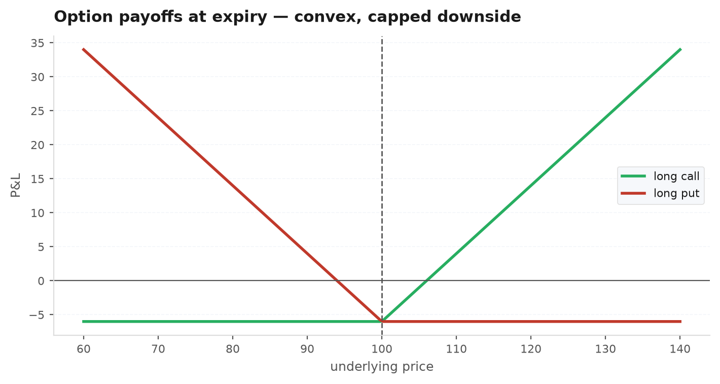
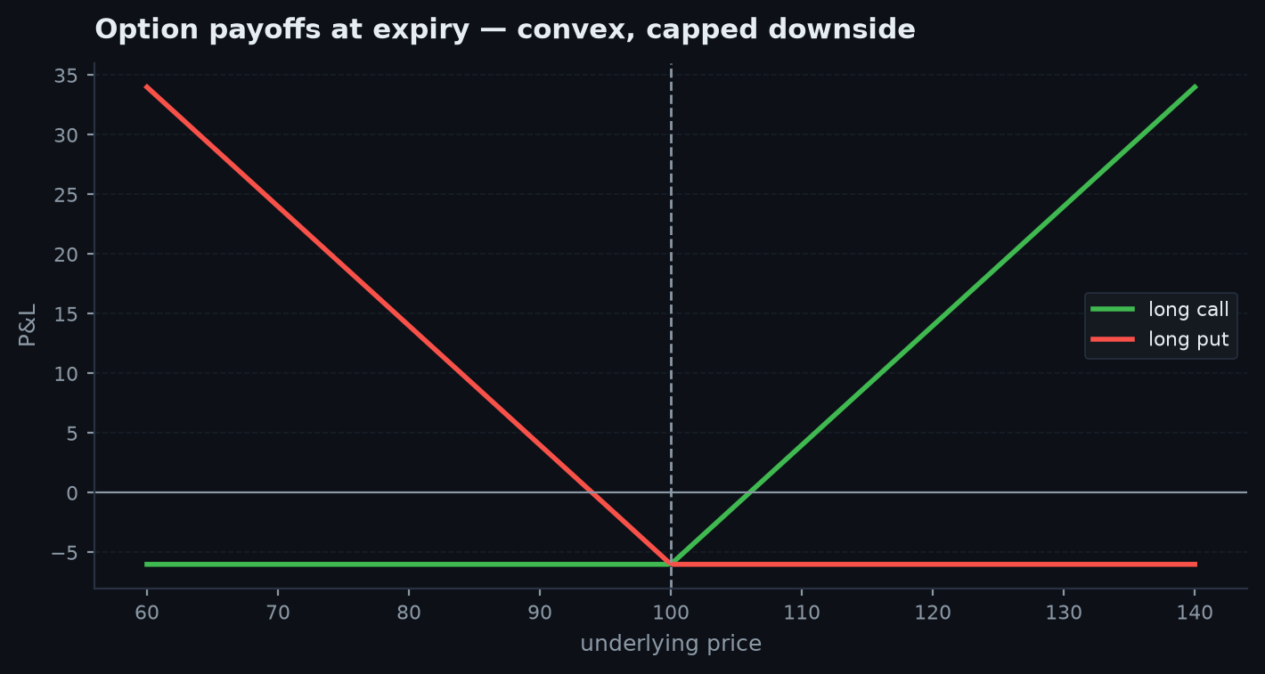
A call pays off when the underlying finishes above the strike; a put pays off below it. At expiry the value depends only on the terminal spot $S_{T}$ and the strike $K$ :

Call_{T} = max (S_{T} - K, 0), Put_{T} = max (K - S_{T}, 0)

The $max (\cdot, 0)$ is the whole story: your loss is floored at the premium you paid, while the upside is open (call) or bounded only by $S_{T} \to 0$ (put). That kinked, convex payoff is what you cannot replicate with the linear P&L of a spot position — it is why options exist.

Payoff diagrams at expiry for a long call and a long put, hockey-stick shapes kinked at the strike — Payoff at expiry. The long call (left) is flat below K then rises 1:1; the long put (right) falls 1:1 toward the strike then flattens. The dashed line subtracts the premium to give profit.

✦Scenario

Buy the Acme $100 call for a $2.30 premium. At expiry your profit is

max (S_{T} - 100, 0) - 2.30

. If earnings disappoint and Acme closes at $95, the call expires worthless and you lose exactly $2.30 — no more, whatever the crash. If it rips to $115 you collect

15 - 2.30 = $12.70

. Your break-even is $102.30 (strike plus premium): below it the trade loses, above it it wins, and the loss can never exceed the premium. That capped, one-sided shape is the convexity a linear share position simply does not have.

Intrinsic value vs time value#

Before expiry an option is worth more than its payoff-if-exercised-now. Split the premium in two:

V = intrinsic max (S - K, 0) + time value (V - max (S - K, 0))

Intrinsic value is what you would collect exercising immediately — zero for an out-of-the-money option. Time value is everything left: the premium the market charges for the chance that the option moves further into the money before expiry. It is largest at-the-money and decays to zero as $t \to 0$ — the erosion that $Θ$ (below) measures.

Scenario. Acme has climbed to $108 and your $100 call now trades at $9.50. Its intrinsic value is $max (108 - 100, 0) = $8$ ; the remaining $9.50 - 8 = $1.50$ is time value — the market's charge for the chance the stock climbs even further before expiry. Hold to the last day with Acme still at $108 and that $1.50 has bled away to nothing: you are left with the $8 intrinsic and not a cent more. The time value is what you are really buying and selling when you trade an option early.

Put-call parity#

Before any pricing model, a pure no-arbitrage relation ties calls and puts together. Consider two portfolios held to expiry $T$ :

A: long one call, short one put, both struck at $K$ . At expiry it is worth $max (S_{T} - K, 0) - max (K - S_{T}, 0) = S_{T} - K$ in every state of the world.
B: long one share (reinvesting the continuous carry $q$ ) plus a loan whose face value is $K$ . At expiry it is worth $S_{T} - K$ too.

Two portfolios with identical payoffs in every state must have identical value today, or you could buy the cheap one, sell the dear one, and pocket a riskless profit. Discounting each leg to the present — the share by its carry, the loan by the rate $r$ — gives put-call parity:

C - P = S e^{- q t} - K e^{- r t}

This holds for European options independent of any model — it never assumes Black-Scholes. It is the first thing to sanity-check a pricer against: price a call and a put at the same strike and confirm the difference equals the forward minus the discounted strike.

parity.py

import numpy as np
import edgekit as ek

S, K, t, r, q, sigma = 100.0, 100.0, 0.5, 0.04, 0.01, 0.20
C = ek.options.bs_price(S, K, t, r, sigma, kind="call", q=q)
P = ek.options.bs_price(S, K, t, r, sigma, kind="put",  q=q)

lhs = C - P
rhs = S * np.exp(-q * t) - K * np.exp(-r * t)
print(round(lhs, 8), round(rhs, 8))   # equal to machine precision

The Black-Scholes price#

Black-Scholes-Merton assumes the underlying follows geometric Brownian motion with constant volatility $σ$ , and prices the option as the discounted expectation of its payoff under the risk-neutral measure (where the drift is the carry-adjusted rate, not the real-world return). The closed form for a call is:

C = S e^{- q t} Φ (d_{1}) - K e^{- r t} Φ (d_{2})

P = K e^{- r t} Φ (- d_{2}) - S e^{- q t} Φ (- d_{1})

where $Φ$ is the standard-normal CDF and

d_{1} = \frac{ln ( S / K ) + ( r - q + \frac{1}{2} σ ^{2} ) t}{σ t}, d_{2} = d_{1} - σ t

Read the call intuitively: $Φ (d_{2})$ is (roughly) the risk-neutral probability of finishing in the money, so $K e^{- r t} Φ (d_{2})$ is the expected cost you pay for the stock, and $S e^{- q t} Φ (d_{1})$ is the discounted expected value of the stock you receive, conditional on exercise. The single free input is $σ$ : everything else is observable. The same formula prices equity ( $q$ = dividend yield), FX ( $q$ = foreign rate) and futures options ( $q = r$ , the Black-76 case).

price.py

import edgekit as ek

# 6-month at-the-money call, 4% rate, 1% carry, 20% vol
px = ek.options.bs_price(S=100, K=100, t=0.5, r=0.04, sigma=0.20, kind="call", q=0.01)
print(round(px, 4))            # ~ 5.9  (all time value: ATM has zero intrinsic)

# deep in-the-money call -> price dominated by intrinsic (S - K discounted)
print(round(ek.options.bs_price(140, 100, 0.5, 0.04, 0.20, kind="call"), 4))

✦Scenario

Back to Acme's earnings bet. Price the 1-month at-the-money call:

S = K = 100

t = 1/12 \approx 0.083

r = 0.04

σ = 0.20

. Black-Scholes returns roughly

$2.30

— the $2.30 premium from the hook, now derived, not assumed. A useful ATM rule of thumb reproduces it:

C \approx 0.4 S σ t = 0.4 (100) (0.20) 0.083 \approx 2.31

. Now stretch the same call to 6 months and the price roughly triples to about $5.90 — twice as much calendar time is not twice the premium, because time value scales with

t

, not

t

. That single square-root is why short-dated options are cheap in dollars but brutally expensive in decay per day.

→Pure numpy, no scipy

ek.options implements

Φ

\frac{1}{2} (1 + erf (x / 2))

via math.erf, so every function is float-in / float-out but also broadcasts elementwise over numpy arrays — price a whole strike ladder in one call by passing an array of K.

The Greeks#

The Greeks are the partial derivatives of the price with respect to each input — the sensitivities you hedge and risk-manage against. ek.options.bs_greeks(...) returns all five in one dict: delta, gamma, vega, theta, rho.

Delta — sensitivity to spot#

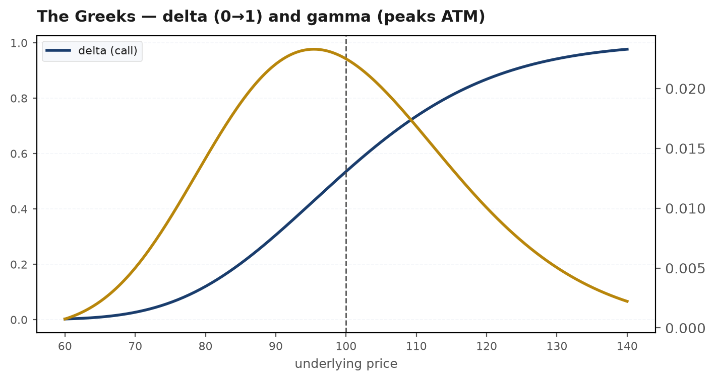
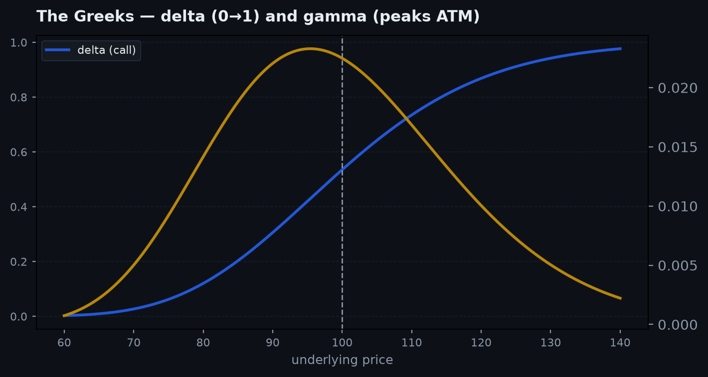
$Δ = \partial V / \partial S$ , the change in option value per $$1$ move in spot. For a call it is exactly:

Δ_{call} = e^{- q t} Φ (d_{1}) \in (0, 1), Δ_{put} = e^{- q t} (Φ (d_{1}) - 1) \in (- 1, 0)

It doubles as the hedge ratio (hold $- Δ$ shares to neutralise spot risk) and as a rough in-the-money probability. Deep ITM calls approach $Δ = 1$ (they behave like stock); far OTM approach $0$ .

Gamma — curvature#

$Γ = \partial^{2} V / \partial S^{2}$ , how fast delta itself moves. It is the same for calls and puts and is always positive for a long option:

Γ = \frac{e ^{- q t} ϕ ( d _{1} )}{S σ t}

Gamma is the convexity you pay theta for. It peaks at-the-money and near expiry, and it is the term that makes a delta-hedged long-option position profit from large moves — the subject of the next chapter.

Vega — sensitivity to volatility#

$V = \partial V / \partial σ$ , the change in value per unit of volatility. Same for calls and puts, always positive for a long option:

V = S e^{- q t} ϕ (d_{1}) t

!Vega is quoted per 1.00 of vol

bs_greeks returns vega per 1.00 (=100 vol-points) of

σ

. To get the more familiar “dollars per 1% vol move”, divide by 100. Likewise theta is per year — divide by 365 for per-calendar-day decay — and rho is per 1.00 of rate (÷100 for per-1%). Getting these unit conventions wrong is the single most common Greeks bug.

Theta — time decay#

$Θ = \partial V / \partial t$ (per year), the erosion of time value as expiry approaches. It is negative for a long option — you bleed premium every day nothing happens:

Θ_{call} = - \frac{S e ^{- q t} ϕ ( d _{1} ) σ}{2 t} - r K e^{- r t} Φ (d_{2}) + q S e^{- q t} Φ (d_{1})

Rho — sensitivity to rates#

$ρ = \partial V / \partial r$ , usually the smallest Greek for short-dated options: $ρ_{call} = K t e^{- r t} Φ (d_{2})$ and $ρ_{put} = - K t e^{- r t} Φ (- d_{2})$ .

Delta, gamma, vega, and theta plotted against spot for a call option, showing delta as an S-curve and gamma/vega peaking at the money — The Greeks as a function of spot. Delta is the S-curve from 0 to 1; gamma and vega both peak at-the-money; theta is most negative where time value (and gamma) is largest.

greeks.py

import edgekit as ek

g = ek.options.bs_greeks(S=100, K=100, t=0.5, r=0.04, sigma=0.20, kind="call", q=0.01)
print(round(g["delta"], 4))          # ~ 0.55  (slightly above 0.5 for ATM call)
print(round(g["gamma"], 5))
print(round(g["vega"] / 100, 4))     # $ per +1% vol  (divide the per-1.00 vega by 100)
print(round(g["theta"] / 365, 4))    # $ per calendar day of decay
print(round(g["rho"] / 100, 4))      # $ per +1% rate

✦At the desk: reading the Acme call's Greeks

Pull the Greeks on the 1-month Acme call (

S = K = 100, t = 0.083, σ = 0.20

) and you get roughly

Δ \approx 0.53

Γ \approx 0.069

, vega

\approx $0.115

per 1% vol, and theta

\approx - $0.043

per day. Read them as a risk report on your $2.30 bet: (1) delta 0.53 — if Acme ticks up $1 the call gains about 53 cents, and to hedge the direction out you would short 0.53 shares per call; (2) gamma 0.069 — after that $1 move delta climbs to

\approx 0.60

, so the position accelerates into the move (the convexity you paid for); (3) vega $0.115— if the market's implied vol jumps from 20% to 25% ahead of earnings, the call gains

5 \times 0.115 \approx $0.58

with the stock unchanged; (4) theta −$0.043 — every quiet day costs you 4.3 cents of premium. Own the call and you are long stock-sensitivity, long convexity, long vol, and short time. That is the whole position in four numbers.

Implied volatility#

Black-Scholes takes $σ$ and returns a price. In the market you observe the price and want the volatility that reproduces it — the implied volatility. Because the price is strictly increasing in $σ$ (vega > 0), there is a unique solution, found by inverting the formula numerically:

find σ_{imp} s.t. BS (S, K, t, r, σ_{imp}, q) = V_{market}

ek.options.implied_vol does this with Newton-Raphson on vega, falling back to bisection when a step leaves the no-arbitrage bracket. It returns nan when no positive vol can reproduce the price — chiefly a quote below intrinsic value, or a non-positive price/time.

iv.py

import edgekit as ek

# price a call at a known vol, then recover that vol from the price
px  = ek.options.bs_price(100, 100, 0.5, 0.04, 0.30, kind="call")
iv  = ek.options.implied_vol(px, 100, 100, 0.5, 0.04, kind="call")
print(round(iv, 6))          # -> 0.30, the round-trip is exact

# a quote below intrinsic has no solution
print(ek.options.implied_vol(0.01, 140, 100, 0.5, 0.04, kind="call"))  # nan

✦Scenario

A week before earnings the Acme $100 one-month call is no longer $2.30 — the screen shows it trading at $2.85. You did not change your rate or the time to expiry, so what does the market know that you did not? Invert it: ek.options.implied_vol(2.85, 100, 100, 0.083, 0.04, kind="call") returns roughly

0.25

. The market is pricing 25% implied vol, not your 20% — it expects the earnings print to shake the stock 25% harder (annualised) than its recent history did. That 5-vol-point gap is the earnings risk premium, made explicit. If you still believe 20% is the right number, the call is expensive and you are on the wrong side of the bet — which is precisely the comparison the next chapter turns into a trade.

Implied vol is the market's forward-looking price of risk, and reading it across strikes and maturities is where the constant- $σ$ assumption of Black-Scholes visibly breaks — the vol smile. That is the door into volatility trading.

Next: Volatility trading — realized versus implied vol, the variance risk premium, the smile, and delta-hedging a long-gamma book.