Volatility trading

Once you can price an option you can trade the one input that is not observable: volatility. A vol trader is not betting on direction — they are betting that the volatility implied by option prices is wrong relative to what the underlying will actually realize. This chapter defines both, explains the persistent gap between them (the variance risk premium), shows why the vol smile proves Black-Scholes is a convenient lie, and then walks through the mechanics — straddles, and the gamma-versus-theta P&L of a delta-hedged position — together with the tail risk that makes short vol so dangerous.

✦Why a trader cares

In the last chapter you found the Acme earnings call was pricing 25% implied vol against your 20% estimate. A vol trader does not ask “will Acme go up?” — they ask “is 25% too high?” If the stock will really only swing at a 20% pace, then whoever sells that 25% vol and hedges out the direction collects the 5-point difference as profit. This chapter is how that bet is expressed, measured, and — because it is one of the most seductive ways to blow up an account — how it kills you when it goes wrong.

Realized vs implied volatility#

Realized volatility is backward-looking: the annualised standard deviation of the returns the underlying actually printed. From log returns $r_{t}$ over a window of $n$ bars with $A$ bars per year:

σ_{realized} = \frac{A}{n} t = 1 \sum n (r_{t} - r ˉ)^{2}

Implied volatility is forward-looking: the single $σ$ you back out of a traded option price with ek.options.implied_vol(previous chapter). It is the market's consensus forecast of volatility over the option's life. In edgekit the realized side comes from ek.timeseries:

realized.py

import numpy as np
import edgekit as ek

logret = np.diff(np.log(close))

# rolling per-bar std, annualised by sqrt(periods_per_year)
rv = ek.timeseries.rolling_volatility(logret, window=20, periods_per_year=252)

# EWMA (RiskMetrics): weights recent shocks more, reacts to regime change
ew = ek.timeseries.ewma_volatility(logret, lam=0.94) * np.sqrt(252)

# realized_vol is the HF estimator: sqrt of the rolling *sum* of squared returns
rvol = ek.timeseries.realized_vol(logret, window=20)

✦Scenario

Over the last 20 trading days the S&P 500 printed daily log-returns with a standard deviation of about 0.72%. Annualise it:

σ_{realized} = 0.0072 \times 252 \approx 11.4%

— a calm tape. Meanwhile the VIX (30-day implied vol on the same index) reads 18%. The index has been realizing 11% while options are implying18%: a 7-point gap. Anyone who sold that 30-day vol and delta-hedged would have banked the difference, because the market delivered far less movement than the premium priced. That persistent “implied sits above realized” wedge has a name.

→Three vol estimators, three jobs

rolling_volatility is the textbook rolling std (a per-bar average). realized_vol is the high-frequency total-variation estimator — the sum of squared returns, larger by roughly

n

, measuring how far the series actually travelled. ewma_volatility replaces the hard lookback window with exponential decay so a new shock is felt immediately. Pick by purpose; do not mix their scales in one comparison.

The variance risk premium#

Compare the two series and a robust empirical fact appears: implied volatility is, on average, higher than the volatility that subsequently realizes. The average gap is the variance risk premium (VRP):

VRP = E [σ_{implied}^{2} - σ_{realized}^{2}] > 0

Why does it persist? Options are insurance. Most participants are natural buyers of protection (long puts, long vol), and the sellers who warehouse that risk demand compensation for taking on rare, violent losses. So implied vol embeds a risk premium above the statistical forecast — the same reason insurance premiums exceed expected claims. Selling vol harvests this premium most of the time, which is exactly what makes it dangerous: the payoff is a long stream of small gains punctuated by rare catastrophic losses.

!A premium is not a free lunch

The VRP is real and well-documented, but this is a tutorial on mechanics, not a trade recommendation. A positive average spread says nothing about whether a specific short-vol structure survives its own tail, its transaction costs, or a regime shift — put any such idea through the gauntlet before believing it.

The vol smile and skew#

Black-Scholes assumes one constant $σ$ for all strikes. If that were true, inverting every option on the same underlying and expiry would yield the same implied vol. It does not. Plot implied vol against strike and you get a smile (or, in equity and index markets, a downward skew): out-of-the-money options — especially downside puts — trade at higher implied vol than at-the-money.

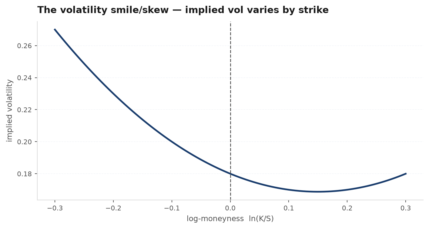
Implied volatility plotted against strike, forming a smile that tilts up more steeply on the downside (skew) — Implied volatility by strike. A flat line is what Black-Scholes predicts; the observed smile/skew — steeper on the downside — is the market pricing fat tails and crash risk that a single constant sigma cannot capture.

The smile is the market correcting Black-Scholes' two false assumptions: returns are not Gaussian (they have fat tails, so far-OTM options are worth more than a normal distribution implies), and volatility is notconstant (it clusters and spikes precisely when prices fall). The downside skew in equities encodes crash-o-phobia: demand for put protection bids up implied vol on the left wing. Practically, the smile means there is no single “the” volatility — you must speak of the implied vol at a given strike, and any model with one $σ$ will misprice the wings.

smile.py

import numpy as np
import edgekit as ek

S, t, r = 100.0, 0.25, 0.04
strikes = np.array([80, 90, 100, 110, 120], float)

# Suppose these are observed market prices for calls at each strike.
# Inverting each with implied_vol recovers a *different* sigma per strike:
market_px = np.array([...])   # traded prices
ivs = [ek.options.implied_vol(px, S, K, t, r, kind="call")
       for px, K in zip(market_px, strikes)]
# a flat 'ivs' would confirm BS; a U-shape is the smile.

✦Scenario

Take one-month options on the S&P 500 with the index at 5000 and invert each traded price to an implied vol. A realistic skew looks like this: the 4500 put (10% out-of-the-money, the crash strike) prints

\approx 24%

; the 5000 at-the-money prints

\approx 18%

; the 5500 call (10% OTM upside) prints only

\approx 15%

. Three strikes on one index and one expiry, three different volatilities — Black-Scholes says they must be identical. The downside puts are the most expensive because that is where the fear (and the demand for crash insurance) lives. Practically: there is no “the vol of the S&P” — you must always say the vol at which strike, and a one-

σ

model will misprice the wings by 5-6 vol points.

Trading volatility with structures#

To bet on the magnitude of a move while staying (initially) direction-neutral, combine options so the deltas cancel and the vega adds.

Straddle and strangle#

A long straddle is a long call plus a long put at the same at-the-money strike. Its deltas roughly offset ( $Δ_{call} + Δ_{put} \approx 0$ at the money), leaving a position that is long gamma and long vega: it profits from a large move in either direction, or from implied vol rising, and it pays for that convexity through theta. A strangle uses OTM strikes instead — cheaper premium, but the underlying must travel further before it pays.

straddle.py

import edgekit as ek

S = K = 100.0; t, r, sig = 0.25, 0.04, 0.25
call = ek.options.bs_price(S, K, t, r, sig, kind="call")
put  = ek.options.bs_price(S, K, t, r, sig, kind="put")
premium = call + put                      # cost of the straddle

gc = ek.options.bs_greeks(S, K, t, r, sig, kind="call")
gp = ek.options.bs_greeks(S, K, t, r, sig, kind="put")
net_delta = gc["delta"] + gp["delta"]     # ~ 0 at the money
net_vega  = gc["vega"]  + gp["vega"]       # additive, long vol
print(round(premium, 3), round(net_delta, 4), round(net_vega / 100, 3))

✦Scenario

A biotech, Zenith Pharma, trades at $100 with an FDA ruling due in three months. You have no view on approval-vs-rejection but you are certain the news will move the stock violently. Buy the 3-month $100 straddle at

σ = 25%

: the call costs about $5.20, the put about $4.30, so the straddle costs roughly

$9.50

. Net delta is near zero (the two legs cancel), so you do not care which way — you care how far. Your break-evens are strike ± premium, i.e. $90.50 and $109.50: Zenith must move more than

\approx 9.5%

in either direction before expiry for the position to pay. A verdict that sends it to $120 nets

20 - 9.50 = $10.50

; a boring $103 close loses most of the premium to theta. You bought movement and vega; the FDA either delivers or you bleed.

Delta-hedging: gamma vs theta#

Buying a straddle leaves you exposed to direction if the underlying drifts. To isolate a pure vol bet, continuously delta-hedge: hold $- Δ$ units of the underlying and rebalance as spot moves. A delta-hedged long option has no first-order spot exposure, so its P&L over a small step $Δ S$ in time $d t$ is the second-order Taylor expansion:

d P \approx \frac{1}{2} Γ (Δ S)^{2} + Θ d t

This is the central identity of vol trading. The first term is positive (long gamma: $Γ > 0$ and $(Δ S)^{2} \geq 0$ ) — you make money from movement regardless of sign, because each rebalance buys low and sells high around the hedge. The second term is negative (theta decay: $Θ < 0$ ) — you bleed time value every day. The net is a race:

d P \approx \frac{1}{2} Γ S^{2} (σ_{realized}^{2} - σ_{implied}^{2}) d t

Rewritten this way it is transparent: a delta-hedged long option makes money exactly when realized volatility exceeds the implied vol you paid, and loses when it does not. You bought vol at $σ_{implied}$ ; the market delivers $σ_{realized}$ ; the difference, scaled by your gamma exposure, is the P&L. The short-vol seller sits on the other side of this equation — collecting theta, praying gamma losses stay small.

✦Scenario: the gamma-vs-theta race, day by day

You delta-hedge the long Zenith straddle. Say it carries

Γ \approx 0.06

and

Θ \approx - $0.08

per day. Set the two terms equal to find your break-even daily move:

\frac{1}{2} (0.06) (Δ S)^{2} = 0.08 \Rightarrow Δ S \approx $1.63

, i.e. a 1.6% day — which annualises to

1.6% \times 252 \approx 25%

, exactly the implied vol you paid. That is not a coincidence; it is the identity above. Now watch two days:
• A 4% day (

Δ S = $4

): gamma earns

\frac{1}{2} (0.06) (4)^{2} = $0.48

, theta costs $0.08, net +$0.40. Movement won.
• A quiet 0.8% day (

Δ S = $0.80

): gamma earns only

\frac{1}{2} (0.06) (0.8)^{2} = $0.02

, theta still costs $0.08, net −$0.06. Time won. Sum a month of days: you profit if and only if Zenith realizes more than the 25% you paid. The hedge turned a directional lottery ticket into a clean bet on realized-vs-implied.

✦The trade IS the variance risk premium

Selling a delta-hedged straddle is the direct expression of the VRP: you collect

Θ d t

and pay out

\frac{1}{2} Γ (Δ S)^{2}

. On average implied > realized, so on average you win — but the loss term is unbounded in a gap, and no amount of average edge saves you from a single day where

(Δ S)^{2}

is huge.

The short-vol tail#

The reason short vol is treated with such caution is the shape of its return distribution: many small positive days (theta collected) and a fat, sudden left tail (gamma losses in a crash, compounded by implied vol spiking against your short vega at the worst moment). It is negatively skewed and leptokurtic — the mirror image of the right-skewed trend-following payoff. Standard risk metrics flatter it: a short-vol book can post a gorgeous Sharpe for years and then surrender it all in a week, because Sharpe cannot see a tail it has not sampled yet.

!Scenario: the short-vol seller who was right until they weren't

Flip the earlier trade around. A desk sells the 30-day S&P vol at 18% while the index realizes 11%, and delta-hedges. Month after month it collects the

Θ d t

spread — a steady

\approx + 1%

a month, Sharpe near 2, a beautiful equity curve. Then a shock hits: the index gaps −6% in a day and implied vol spikes from 18% to 45%. The gamma term

\frac{1}{2} Γ (Δ S)^{2}

— now with the sign against them — detonates, and the short vega loses again as implied vol reprices upward at the worst possible moment. One day erases eighteen months of premium. The average edge was real; it just never paid for the tail. Size against that day, not against the Sharpe.

This is not a reason to avoid vol — it is a reason to size it against the tail, not the average. The lessons from position sizing and Monte Carlo apply with full force: bootstrap the worst case, never let a single event exceed your ruin threshold, and report MAR and the loss distribution alongside any headline return.

Next: Market microstructure — the limit order book, the anatomy of the bid-ask spread, and where trading costs are actually born.