Returns & compounding

Before any strategy, edge, or backtest, you need to measure change correctly. Two ways to write down a return look almost identical and behave completely differently once you chain them together. Getting this wrong quietly corrupts every metric downstream — Sharpe, CAGR, drawdown — so we start here.

Simple returns#

The simple (arithmetic) return over one period is the fractional change in price. If $P_{t}$ is the close at time $t$ :

r_{t} = \frac{P _{t}}{P _{t - 1}} - 1 = \frac{P _{t} - P _{t - 1}}{P _{t - 1}}

A move from 100 to 110 is $r = 0.10$ — a 10% return. This is the number you actually earn on capital over the period, which is exactly why it is the right unit for combining across assetsat a point in time: a portfolio’s simple return is the weighted sum of its holdings’ simple returns.

!Simple returns do not add across time

Up 10% then down 10% is not flat.

1.10 \times 0.90 = 0.99

— you are down 1%. Percentages you can average in your head are lying to you the moment you chain periods together.

Log returns#

The log (continuously-compounded) return is the natural log of the price ratio:

ℓ_{t} = ln (\frac{P _{t}}{P _{t - 1}}) = ln P_{t} - ln P_{t - 1}

For small moves the two are nearly equal — $ln (1 + r) \approx r$ when $r$ is small — so a 1% day is ~0.00995 in log space. The difference only bites on big moves and over long chains. The reason log returns matter is one property:

Why log returns add#

Because the log of a product is the sum of the logs, the multi-period log return is just the sum of the single-period log returns:

ℓ_{0 \to T} = ln (\frac{P _{T}}{P _{0}}) = t = 1 \sum T ln (\frac{P _{t}}{P _{t - 1}}) = t = 1 \sum T ℓ_{t}

→Derivation — the telescoping product

Start from the identity that the intermediate prices cancel. Write the terminal price ratio as a product of the single-period ratios:

\frac{P _{T}}{P _{0}} = \frac{P _{1}}{P _{0}} \cdot \frac{P _{2}}{P _{1}} \cdot \frac{P _{3}}{P _{2}} \dots \frac{P _{T}}{P _{T - 1}} = t = 1 \prod T \frac{P _{t}}{P _{t - 1}}

Every $P_{t}$ for $1 \leq t \leq T - 1$ appears once in a numerator and once in a denominator, so they cancel — that is the “telescope.” Now take $ln$ of both sides and use $ln (ab) = ln a + ln b$ , which turns the product into a sum:

ln (\frac{P _{T}}{P _{0}}) = ln (t = 1 \prod T \frac{P _{t}}{P _{t - 1}}) = t = 1 \sum T ln (\frac{P _{t}}{P _{t - 1}}) . ■

That telescoping is the whole point. Compounding, which is multiplicative in simple returns, becomes plainaddition in log space. Sums of many terms are exactly what the central limit theorem and every variance calculation are built for, so almost all statistics — mean, standard deviation, the Normal approximation — are done on log returns, then converted back at the end.

Property	Simple return	Log return
Aggregate across assets (one period)	Adds (weighted) — use this	Does not add cleanly
Aggregate across time	Multiplies	Adds — use this
Symmetric around zero	No (+10% ≠ −10%)	Yes
Bounded below	≥ −100%	Unbounded (−∞ possible)

→The rule of thumb

Combine across assets in simple returns; combine across time in log returns. Mixing them up is one of the most common silent bugs in a backtest.

Arithmetic vs geometric mean#

Given a series of simple returns, you can summarise them two ways. The arithmetic mean is the plain average:

r ˉ_{arith} = \frac{1}{T} t = 1 \sum T r_{t}

The geometric mean is the constant per-period rate that reproduces the actual ending wealth:

r ˉ_{geom} = (t = 1 \prod T (1 + r_{t}))^{1/ T} - 1

The geometric mean is what you actually compound at; the arithmetic mean is what you would expect on the next single period. They are equal only when every return is identical, and otherwise the geometric mean is always smaller. The gap between them is caused by volatility — and that gap has a name.

Proof: the geometric mean never exceeds the arithmetic mean#

Write the gross returns $a_{t} = 1 + r_{t} > 0$ . The claim $GM \leq AM$ is the classical AM–GM inequality. The cleanest one-line argument uses the concavity of the logarithm.

→Derivation — AM ≥ GM via a concave log

The function $ln$ is concave (its second derivative $- 1/ x^{2}$ is negative everywhere). Jensen’s inequality for a concave function says the function of the average is at least the average of the function. Apply it to the $T$ gross returns, each weighted $1/ T$ :

ln AM \frac{1}{T} t = 1 \sum T a_{t} \geq \frac{1}{T} t = 1 \sum T ln a_{t} = ln GM (\prod_{t = 1}^{T} a_{t})^{1/ T}

Because $ln$ is strictly increasing, we can drop it from both sides without flipping the inequality:

\frac{1}{T} t = 1 \sum T a_{t} \geq (t = 1 \prod T a_{t})^{1/ T} ⟺ AM \geq GM . ■

Equality holds only when all $a_{t}$ are equal — i.e. a perfectly flat return stream. Any dispersion at all pushes GM strictly below AM.

✦Why it matters for trading

The arithmetic mean is the number a naive backtest average reports; the geometric mean is the number your account actually grows at. Quoting the arithmetic mean of a volatile strategy overstates real compounded growth — and the noisier the returns, the bigger the lie. Always judge a strategy by its geometric rate (CAGR), never by the average of its periodic returns.

Compounding & CAGR#

Wealth compounds multiplicatively. Starting from $V_{0}$ , after $T$ periods:

V_{T} = V_{0} t = 1 \prod T (1 + r_{t})

The Compound Annual Growth Rate collapses that whole path into the single annualised rate that would have produced the same ending value (with $T$ measured in years):

CAGR = (\frac{V _{T}}{V _{0}})^{1/ T} - 1

CAGR is a geometric mean by another name, so it is honest about the round-trip: a strategy that doubles then halves has a CAGR of 0%, which is exactly right. This is the number edgekit.metrics.equity_stats reports as cagr.

✦Scenario: the two-year account that fools you

Your account starts at $100,000. Year 1 is great:

+ 50%

, taking it to $150,000. Year 2 gives some back:

- 30%

, leaving

150, 000 \times 0.70 = $105, 000

. The arithmetic mean of your two annual returns is

(50% - 30%) /2 = + 10%

— a number a careless report would headline. But your money grew only 5% total over two years, so the rate you actually compounded at is

CAGR = (105, 000/100, 000)^{1/2} - 1 \approx 2.47%

. The 10% is a fiction; the 2.47% is what is in your account. That gap — 10% down to 2.5% — is what volatility does to compounding, and it only widens with wilder swings.

cagr.py

import numpy as np
from edgekit.metrics import equity_stats

# daily simple returns -> ending wealth and annualised rate
V0, VT = 100_000, 138_400
years = 2.5
cagr = (VT / V0) ** (1 / years) - 1        # -> 0.1357  (13.6%/yr)

es = equity_stats(daily_returns)           # fractional daily returns
print(es["cagr"], es["max_dd_pct"], es["mar"])

Volatility drag#

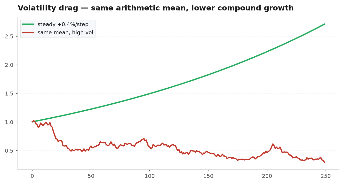
Here is the result that trips up newcomers. The rate you compound at is not your average return — it is your average return minus a penalty for variance. To a good approximation, the geometric growth rate $g$ is:

g \approx μ - \frac{σ ^{2}}{2}

where $μ$ is the arithmetic mean return and $σ$ its standard deviation (both per period). The term $σ^{2} /2$ is volatility drag: the mathematical cost of bouncing around. It falls straight out of the second-order Taylor expansion of $ln (1 + r)$ — the same reason the geometric mean sits below the arithmetic one.

Where the σ²/2 comes from#

The geometric growth rate is the expected log return, $g = E [ln (1 + r)]$ — the per-period version of the additive log return we derived above. Expand the log to second order and take expectations.

→Derivation — second-order expansion

Taylor-expand $ln (1 + r)$ around $r = 0$ :

ln (1 + r) = r - \frac{r ^{2}}{2} + \frac{r ^{3}}{3} - \dots

Take the expectation term by term, keeping to second order:

g = E [ln (1 + r)] \approx E [r] - \frac{1}{2} E [r^{2}]

Now use the variance identity $E [r^{2}] = Var (r) + (E [r])^{2} = σ^{2} + μ^{2}$ :

g \approx μ - \frac{1}{2} (σ^{2} + μ^{2}) \approx μ - \frac{σ ^{2}}{2}

The last step drops $μ^{2}$ : for a per-period return, $μ$ is small and $μ^{2}$ is negligible next to the variance $σ^{2}$ . What survives is the drag term. ■

There is a second, assumption-free way to see the same inequality: Jensen’s inequality. For any concave function $f$ , $E [f (X)] \leq f (E [X])$ . Because $ln$ is concave, applying it with $X = 1 + r$ gives

g = E [ln (1 + r)] \leq ln (E [1 + r]) = ln (1 + μ) \approx μ

so the compounded growth rate can never exceed the arithmetic mean — the drag is exactly the size of that Jensen gap, and it is zero only when $σ = 0$ . This is the same fact as $GM \leq AM$ above, now stated in expectation.

The intuition: a loss hurts more than the same-size gain helps, because after a loss you compound from a smaller base. Down 50% needs a +100% recovery just to break even. Two strategies with the same average return but different volatility do not end up in the same place — the wilder one lags, and the gap widens with time.

✦Scenario: same average, opposite fates

Two strategies each average

+ 1%

per month arithmetically. Steady earns exactly

+ 1%

every month. Wild alternates

+ 21%

and

- 19%

— same arithmetic mean of

+ 1%

. After two months Steady is at

1.0 1^{2} = 1.0201

(up 2.0%), while Wild is at

1.21 \times 0.81 = 0.9801

— down 2.0%, despite the identical average. The

- 19%

month compounds off a base already inflated by the

+ 21%

, so it bites harder. Wild’s per-period variance is about

σ^{2} = 0.2 0^{2} = 0.04

, so the drag

σ^{2} /2 \approx 2%

per month — exactly the shortfall you see. Same headline return, and one grows while the other bleeds.

Two equity curves with equal arithmetic mean but different volatility diverging over time — Same arithmetic mean return, different volatility. The higher-variance path compounds more slowly — the shaded gap is volatility drag, roughly σ²/2 per period.

✦Why this reframes the whole game

Volatility drag is why reducing variance is not just about comfort — it directly raises the rate you compound at. It is the mathematical justification for position sizing, vol-targeting, and diversification: they are all ways to shrink

σ^{2}

and claw back growth. See Position sizing and edgekit.sizing.

Where edgekit measures this#

Two summary builders in edgekit.metrics speak these two languages. Trade-level analysis lives in R-multiples (return normalised by risk — the subject of The math of edge); equity-curve analysis lives in returns and compounds them into CAGR.

two_lenses.py

from edgekit import trade_stats
from edgekit.metrics import equity_stats

# Per-trade lens: expectancy in R, profit factor, MAR
st = trade_stats(trades.r, dates=trades.date)
print(st["ev_r"], st["pf"], st["mar"])

# Equity-curve lens: compounded growth and the drawdown it cost
es = equity_stats(daily_pnl_dollars, account=100_000)
print(es["cagr"], es["max_dd_pct"])

Notice equity_stats reports mar (CAGR divided by max drawdown) alongside cagr. That ratio is the honest one: it asks not just how fast you grew, but how much of a stomach-churning drawdown you had to survive to get there — the volatility-drag lesson turned into a scorecard.

Next: returns are random, so to reason about them we need the language of chance — Probability & distributions.