Backtesting pitfalls — why backtests lie

Almost every apparent edge is an artefact. Before any statistical test, a backtest can already be wrong in five structural ways — and each one produces a beautiful equity curve. This chapter names them, shows how each fools you, and points at the edgekit machinery that guards against it. Learn to distrust your own number first.

Here is the uncomfortable way to hold this: the prettier the equity curve, the more suspicious you should be. A curve that climbs from the bottom-left to the top-right with barely a wobble almost never means "I found a great edge" — it means "I made one of the five mistakes below." Each mistake has a signature look, a story of exactly how it fools a careful person, and a specific edgekit tool built to catch it. Learn the signatures and you learn to flinch at your own good news.

✕The prime directive

Assume every edge is fake until proven otherwise. A good backtest is the start of skepticism, not the end. Your job is to try to break your own strategy before the market does it for you.

1. Look-ahead bias — the classic killer#

Look-ahead is using information at bar $i$ that was not knowable until bar $i + 1$ or later. It is the single most common and most catastrophic error, because it can be as subtle as forgetting to shift one array by one bar.

How it fools you#

Suppose you compute a 20-bar high and enter when the close exceeds it. If the rolling max includes the current bar, the current close is compared to a high that already contains itself — the signal fires with knowledge of the very bar it trades on. The equity curve looks superb: you are, in effect, buying things you already know went up. A single unshifted indicator can add tens of percent of pure fiction.

✦Scenario — the SMA cross that peeked

You code a moving-average cross on BTCUSDT H4: go long when the fast SMA is above the slow SMA. The backtest prints CAGR 41%, PF 1.9 — you are already mentally spending it. Then a colleague asks which bar the SMAs are computed on. You realise your entry reads sma_fast[i] and sma_slow[i] — the values that include bar

i

's own close, the bar you then trade on. You add one line, ek.lag(sma_fast, 1), so the decision only sees through bar

i - 1

. Re-run: CAGR 41% collapses to 6%, PF 1.9 to 1.05. The 35 points of CAGR were never in the market — they were you buying the close of a bar after seeing it close.

!A real project number was ~90% look-ahead

A "+34% improvement" in this project turned out to be roughly 90% look-ahead. This is not a beginner mistake you grow out of — it is a permanent hazard you build guards against.

How edgekit guards it#

The engine enforces causality by construction: indicators are returned unlagged, the caller lags with ek.lag(x, 1) inside prepare, and fills happen at the next open, gap-aware. A decision on bar $i$ can only read through bar $i - 1$ . A CI property test perturbs a future bar and asserts the past does not move — if it does, an indicator is peeking.

lag.py

import edgekit as ek

upper, lower = ek.indicators.donchian(bars.high, bars.low, 20)
upper = ek.lag(upper, 1)          # a decision at bar i may only see through i-1
# entry acts on upper[i]; engine fills at max(level, open[i+1]) for longs

2. Data snooping and overfitting#

Try enough rules, parameters, or filters on one dataset and something will look good by chance alone. This is data snooping — and its close cousin, overfitting, is fitting a rule so tightly to past noise that it describes the history perfectly and predicts nothing.

How it fools you#

If you test $m$ independent strategies with true edge zero, the expected maximum Sharpe among them grows with $m$ — the best of many coin-flippers looks like a genius. The equity curve of the winner is real; what is fake is the belief that it will continue. Every knob you turn, every variant you discard, is a hidden trial that inflates the survivor.

✦Scenario — 50 filters, one winner, zero edge

You bolt filters onto an ORB on US100: session-of-day, an RSI gate, a volatility band, a day-of-week screen — 50 combinations in an afternoon. One of them, "only trade Tue–Thu when RSI < 60", shows Sharpe 1.6 while the raw system sits near 0. It feels like discovery. But with 50 zero-edge coin-flippers, the expected bestSharpe from noise alone is already well above 1 — you did not find a signal, you found the luckiest of 50 dice. The tell: that config sits on a knife-edge (RSI < 55 or < 65 both die), and it fails deflated Sharpe the moment you honestly report n_trials = 50.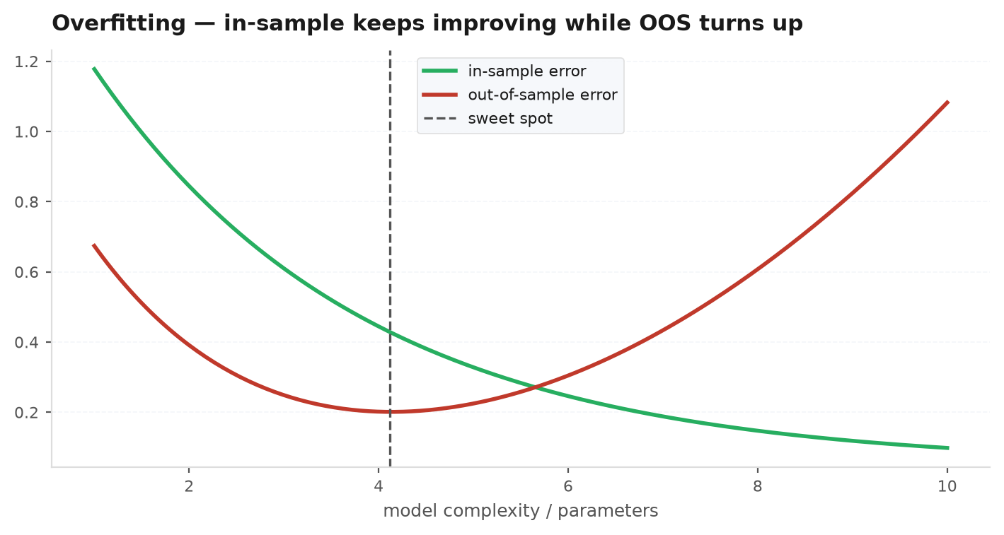

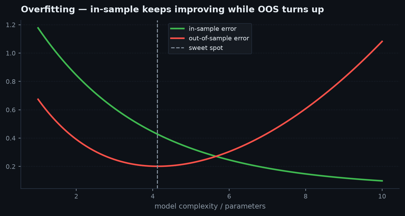
In-sample fit improving while out-of-sample performance degrades as model complexity rises — As you add parameters, in-sample fit keeps improving while out-of-sample performance turns over — the signature of overfitting.

How edgekit guards it#

param_sweep — a real effect is a smooth plateau across its knobs; a lone towering spike at one lucky value is overfit. It reports min / median / max Sharpe and the spread.
pbo_cscv — the Probability of Backtest Overfitting: over every balanced train/test split it checks whether the in-sample-best config lands in the bottom half out-of-sample. Above 0.50 your selection has no OOS power.
deflated_sharpe — discounts the observed Sharpe by the expected maximum Sharpe under the null across n_trials. Report the number of configs you actually tried, honestly.

These get a full treatment in Overfitting detection. The cheapest defence is a strong economic prior: prefer effects with an ex-ante reason to exist over patterns mined from the data.

3. Survivorship bias#

Backtest a universe as it exists today and you have silently excluded everything that died. The delisted, the bankrupt, the merged-away — all gone from your data, all of them losers you never had to hold.

How it fools you#

A mean-reversion rule that "buys the dip" looks wonderful on a survivor-only universe: every name in the sample eventually recovered, because the ones that did not recover were deleted. The strategy that would have caught the falling knives is invisible. The same trap hits index-membership rules, backfilled crypto listings, and any "top N by market cap today" screen applied to the past.

✦Scenario — the altcoin dip-buyer that only saw the winners

You pull the top-30 crypto names as of todayand backtest "buy any 40% drawdown, hold to recovery". It shows a 95% hit rate — nearly every dip recovered. Of course it did: the coins that dropped 40% and never came back (the delisted, the rug-pulled, the −99% zombies) are not in a today-constructed top-30. Your sample was built by the very outcome you are testing. Rebuild the universe point-in-time — every coin that was top-30 at the time of the dip, survivors and corpses alike — and the hit rate falls into the 50s and the "edge" is gone.

How edgekit guards it#

edgekit is single-instrument and point-in-time by design — you feed it one OHLC frame through ek.data, and there is no cross-sectional universe to quietly curate. The discipline is on you: use point-in-time data, include the dead names, and never let a constructed-today universe stand in for what you could actually have traded then.

4. Regime dependence#

A strategy can be genuinely profitable in one market state and quietly lose in another. If your sample is dominated by the favourable regime — a long bull run, a single volatile year — the average looks like an edge when it is really a bet on that regime repeating.

How it fools you#

A trend follower tested only through a bull market shows a gorgeous curve; it is long-biased beta, and it will give it all back in the bear it never saw. A chop-loving mean-reverter tested through a quiet year inverts and bleeds the moment a trend arrives. The blended average hides the fact that the edge lives entirely in one state.

✦Scenario — a trend follower that was just 2020–21 in disguise

Your BTCUSDT Donchian breakout shows +180% total, PF 1.7 over 2019–2025. Impressive — until you split it by year with regime_by_year. The breakdown: 2020 +85R, 2021 +60R, and then 2022 −18R, 2023 +4R, 2024 +6R, 2025 −3R. Nearly the entire result lived in the two roaring bull years; strip them and the strategy is roughly flat-to-negative. That is not a durable edge, it is a long-only bet that 2020–21 repeats. The honest read is "profitable in strong uptrends, bleeds slowly otherwise" — useful to know, but you size it as the regime bet it is, not the all-weather system the blended average pretended to be.

How edgekit guards it#

regime.py

import edgekit as ek

# per-year breakdown — is the edge spread across years, or one lucky one?
by_year = ek.validation.regime_by_year(trades.r, trades.date)
print(by_year[["n", "ev", "win", "pf", "total_r"]])

# trend vs chop, split on ADX — a trend system should earn in trends, bleed little in chop
adx   = ek.indicators.adx(bars.high, bars.low, bars.close, 14)
split = ek.validation.regime_by_adx(bar_net_r, adx, thr=20.0)
print(split["trend_ev"], split["chop_ev"])

The walk-forward test is the stronger version: it demands the edge show up in block after block through time, including the ugly regimes, not just on average.

5. Cost sensitivity#

Many "edges" are alive only inside an optimistic cost assumption. Halve the spread you assumed and the curve soars; double it — closer to what you actually pay — and the whole thing collapses.

How it fools you#

High-frequency and mean-reversion rules are especially fragile: they trade often, so a few basis points per round trip compound into the difference between profit and ruin. A backtest at zero or nominal cost can show a profit factor comfortably above 1 that lives entirely in the space between the assumed spread and the real one.

How edgekit guards it#

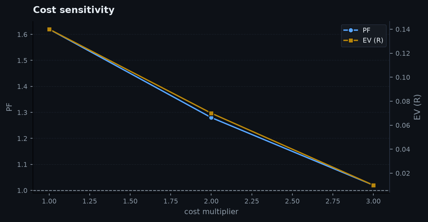
cost_stress re-runs the strategy at 1×, 2×, and 3× cost. The survivor rule: profit factor must stay above 1 at 2× and 3×. If it drops below 1 the moment you double the spread, the edge was living inside the cost assumption, not the market.

✦Scenario — the scalper that dies at 2× spread

A 5-minute mean-reversion system on US100 trades ~1,400 times/year and shows PF 1.22 at your assumed 0.6-point spread. Looks bankable. You run cost_stress: at 1× spread PF 1.22, at 2× (1.2 points — closer to what you actually get filled at in fast tape) PF 0.97, at 3× PF 0.81. The edge was 22% above break-even and the realistic spread ate all of it. Compare a swing trend system trading 40 times/year: PF 1.5 → 1.42 → 1.35 across the same sweep. Same survivor rule, opposite verdict — the scalper is rejected here, the swing system walks on to the next gate.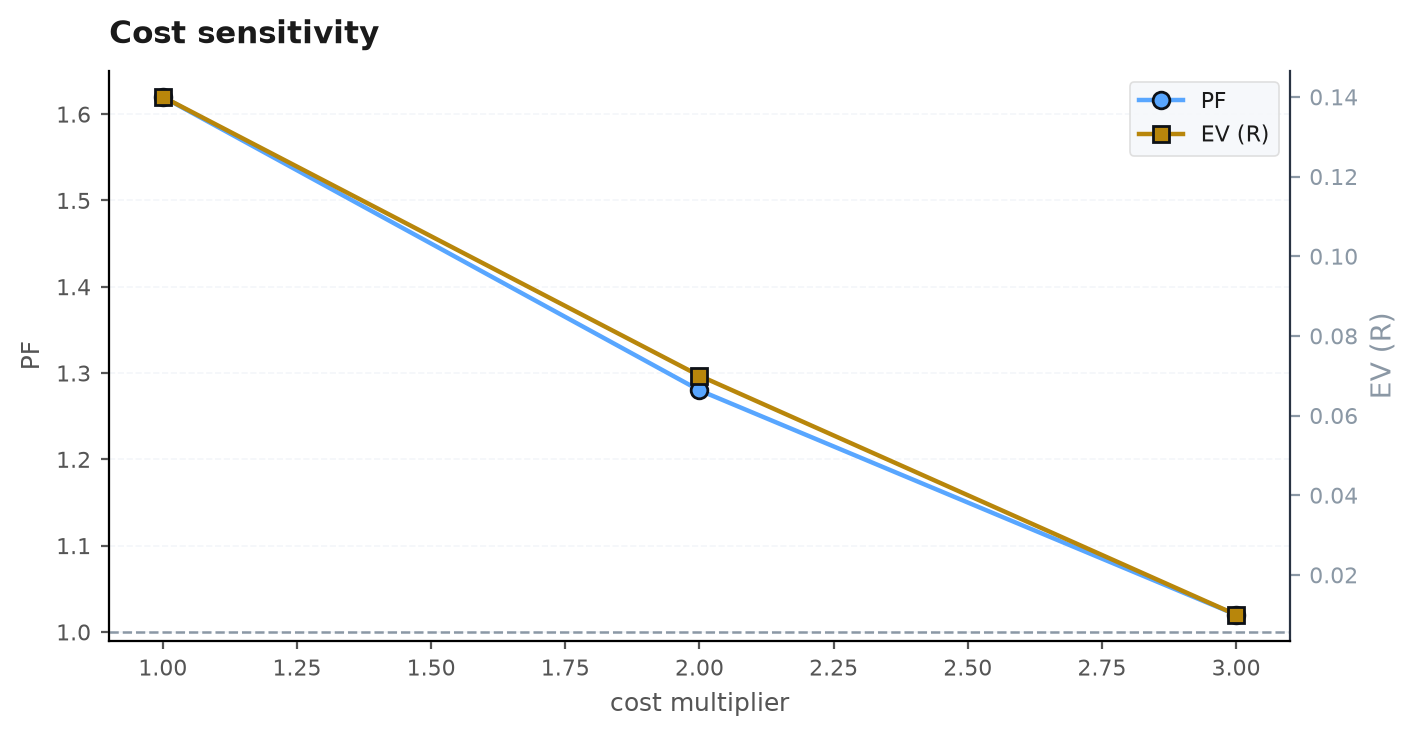

Profit factor falling as the cost multiplier rises from 1x to 3x — A cost-sensitivity sweep: a real edge degrades gracefully; a fake one crosses below PF = 1 as soon as costs rise.

cost_stress.py

import edgekit as ek

def run(cost):
    trades = ek.engine.run_bar_loop(bars, strategy, cost=cost)
    return ek.trade_stats(trades.r)

grid = ek.validation.cost_stress(run, base=ek.costs.CostModel(), mults=(1.0, 2.0, 3.0))
for mult, stats in grid.items():
    print(mult, "x -> PF", round(stats["pf"], 2))   # want > 1 at 2x and 3x

✦The through-line

Look-ahead is caught by construction, snooping by the overfit battery, survivorship by point-in-time data, regime dependence by the year/ADX and walk-forward splits, and cost sensitivity by the stress harness. The gauntlet is just these guards run in a fixed order. Stop believing at the first failure.

Next: Performance metrics — the formulas for the numbers you will judge an edge on, and which of them lie to you about trend-following.