Performance metrics

Every metric compresses an equity curve into one number, and every compression throws something away. This chapter gives the formula for each headline statistic, the assumption it smuggles in, and the exact key it maps to in ek.metrics. The recurring lesson: no single number is safe to judge an edge on — report profit factor and MAR alongside Sharpe, always.

Think of it like a doctor reading vitals. No single reading tells you whether the patient is healthy — a great pulse means nothing if the blood pressure is a disaster. Each metric below is one vital sign of an equity curve, and each has a blind spot the others cover. The skill is not memorising formulas; it is knowing which number lies about which kind of strategy, so you always read them in a group. To make that concrete, we will carry one small, real-looking set of trades through the trade-level metrics and compute them by hand.

Trade-level metrics#

These summarise a stream of per-trade R-multiples. In edgekit they come from ek.trade_stats(r, dates=...), which returns a dict; the key for each is called out below.

→The worked trade set

Ten closed trades from a trend system, in R: [−1, −1, +2.4, −1, +0.5, −1, +3.1, −1, −1, +1.6]. Six losers (all stopped at −1R), four winners. We will compute win rate, expectancy, and profit factor on exactly these ten numbers below — the same numbers ek.trade_stats would return.

Win rate#

The fraction of trades that made money. Alone it is nearly meaningless — a 90%-win-rate strategy that risks 10 to make 1 is a slow-motion disaster.

W_{rate} = \frac{# { r _{i} > 0 }}{N}

Key: win_rate. Read it only in the same breath as average win and average loss (avg_win, avg_loss).

On our set. 4 of 10 trades made money, so the win rate is $4/10 = 0.40$ — a losing-looking 40%. Held up alone it says "this system loses more often than it wins" and you might kill it on the spot. That would be a mistake, as expectancy shows next: this is a trend system, and trend systems are supposed to win less than half the time.

Expectancy#

The expected R per trade — the single most important trade-level number. It is the win rate and payoff woven together:

E [R] = p W - (1 - p) L

where $p$ is win probability, $W$ the average win in R, and $L$ the average loss in R. Positive expectancy is the necessary condition for an edge; everything else is about how reliably and how fast it compounds. Key: ev_r.

On our set. The winners average $W = (2.4 + 0.5 + 3.1 + 1.6) /4 = 1.9$ R and the losers average $L = 1.0$ R, with $p = 0.40$ . So $E [R] = 0.40 \times 1.9 - 0.60 \times 1.0 = 0.76 - 0.60 = + 0.16$ R per trade. (Identical to just averaging all ten: $1.6/10 = + 0.16$ R.) That flips the verdict the 40% win rate implied: despite losing 60% of the time, the system earns +0.16R every time you pull the trigger, because the winners are nearly twice the size of the losers. This is the number that actually decides "is there an edge" — and the reason you never kill a strategy on win rate alone.

Profit factor#

Gross win divided by gross loss — the most robust single summary of an edge. It survives skew, assumes nothing about normality, and is the number you cost-stress against.

PF = \frac{\sum _{r_{i} > 0} r _{i}}{\sum _{r_{i} < 0} r _{i}}

$PF = 1$ is break-even; below 1 the strategy loses. It returns $\infty$ when there are no losing trades. Key: pf (also standalone as ek.profit_factor).

from edgekit import profit_factor
profit_factor([2.0, -1.0, -1.0])   # -> 1.0  (2 won / 2 lost)
profit_factor([1.0, 1.0])          # -> inf  (no losers)

On our set. Gross win is $2.4 + 0.5 + 3.1 + 1.6 = 7.6$ R; gross loss is the six −1R stops, $6.0$ R. So $PF = 7.6/6.0 = 1.27$ . Read that as "for every dollar the system loses, it makes 1.27" — a modest but genuine edge. Now the three trade-level vitals together tell one coherent story instead of three contradictory ones: win rate 0.40 (loses often), expectancy +0.16R (but wins bigger), profit factor 1.27 (net positive, net of cost). Any one in isolation misleads; the trio does not. And 1.27 is the number you now hand to cost stress — if it sinks below 1.0 at 2× spread, the edge was living in the cost assumption.

The R-multiple distribution#

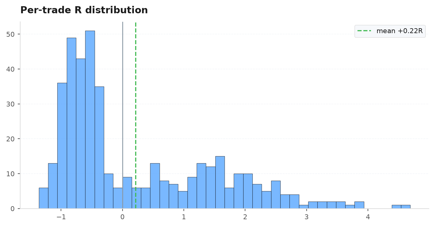
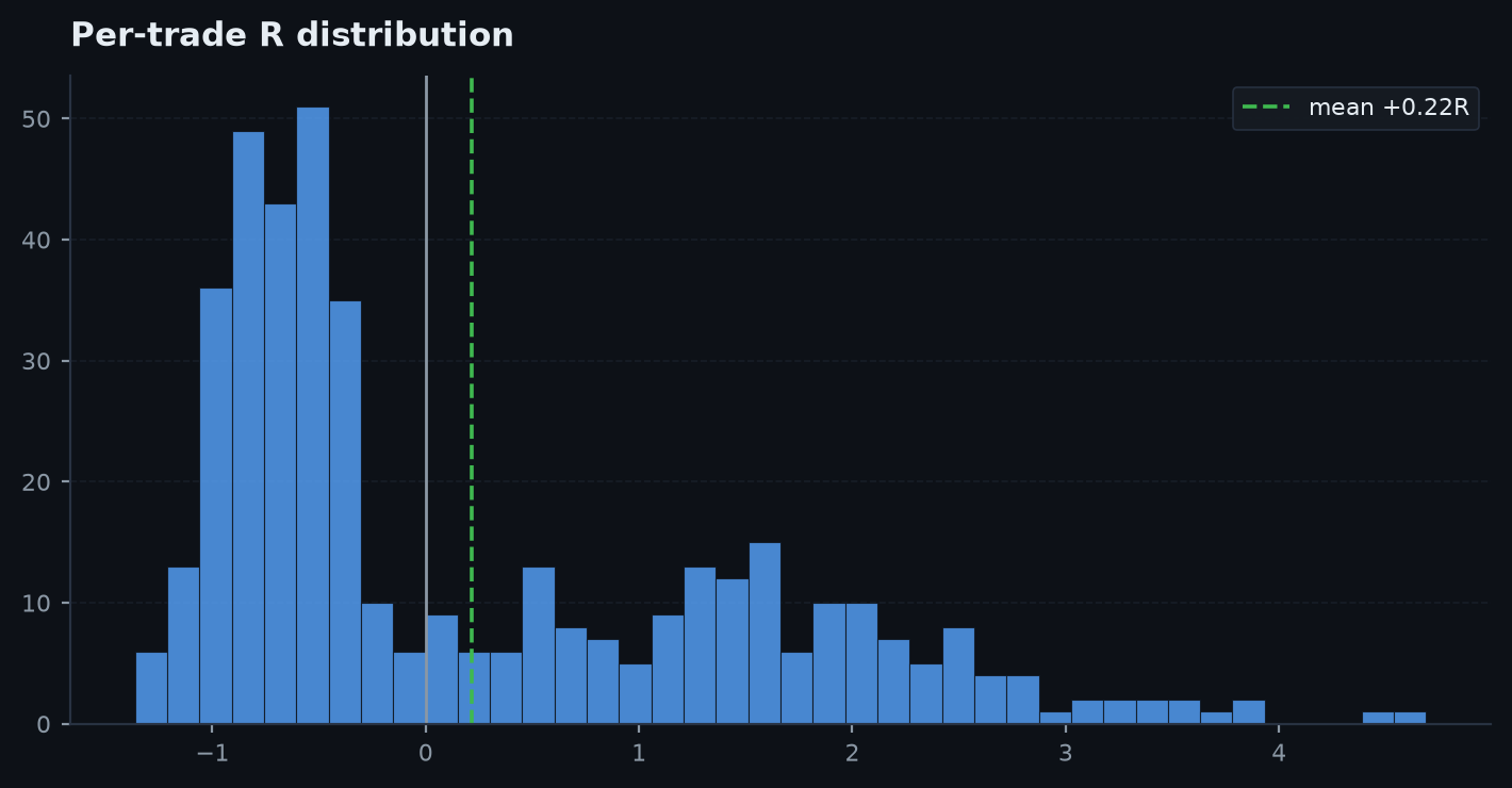
Before trusting any summary, look at the shape. A histogram of per-trade R exposes what the averages hide: fat tails, a cluster of −1R stops, the handful of big winners a trend system lives on. Trend-following R is right-skewed — many small losers, few large winners — which is exactly why Sharpe (below) understates it.

Histogram of per-trade R-multiples with a cluster near −1R and a right tail of winners — Per-trade R-multiples. The stop clusters losses near −1R; the right tail is where a trend edge earns its expectancy.

Equity-curve metrics#

These summarise a daily P&L or return series. In edgekit they come from ek.metrics.equity_stats(daily_pnl, account=...); the trade summary also surfaces the R-space versions when you pass dates.

CAGR#

The compound annual growth rate — the constant yearly rate that would take $V_{0}$ to $V_{T}$ over $T$ years:

CAGR = (\frac{V _{T}}{V _{0}})^{1/ T} - 1

Key: cagr (from equity_stats); the R-space annualised return is ann_r (from trade_stats with dates).

Maximum drawdown#

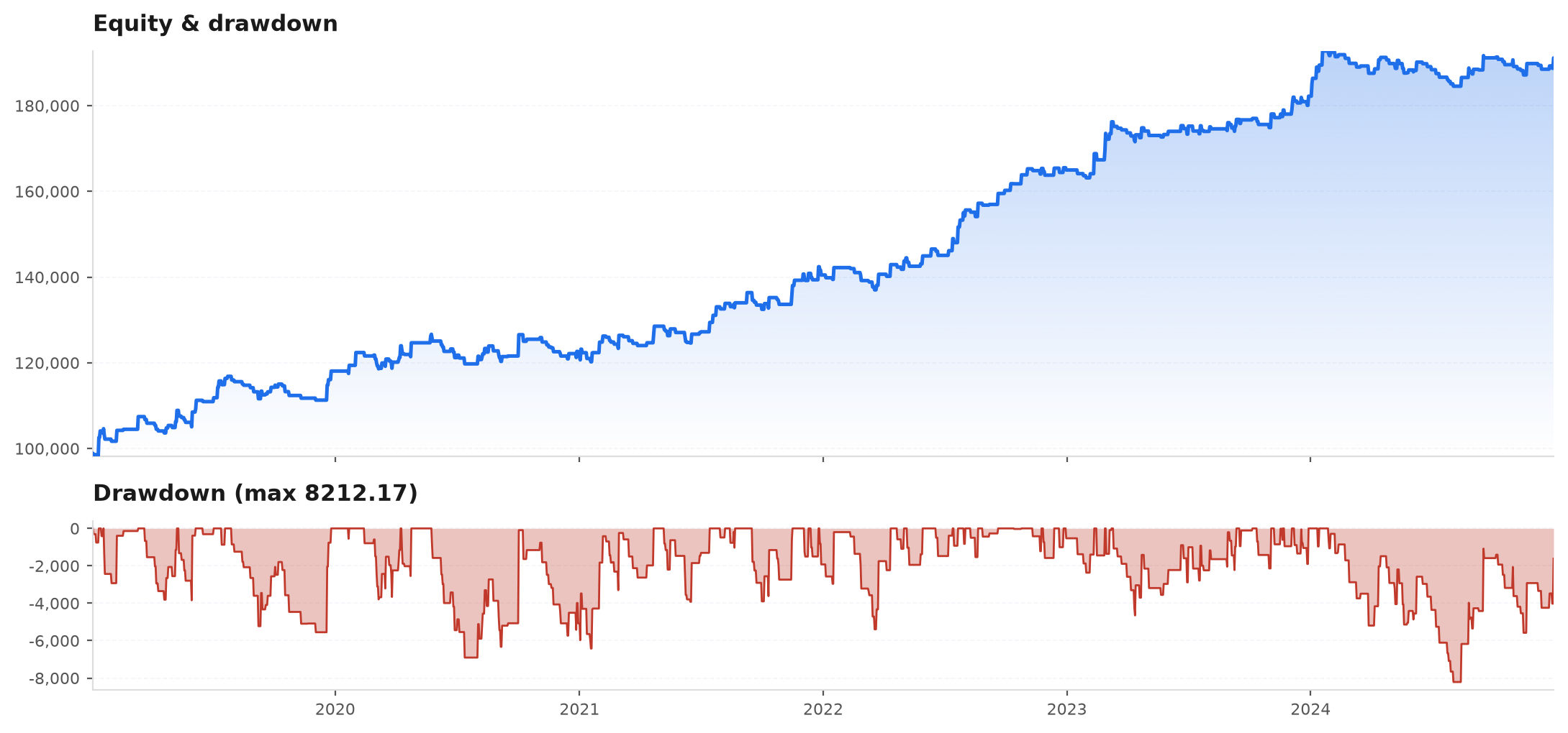
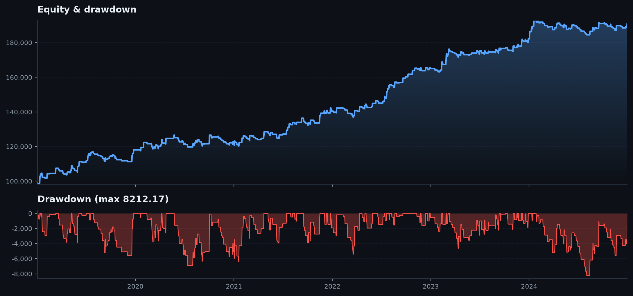
The largest peak-to-trough decline the equity curve ever suffered — the metric that decides whether you can actually hold the strategy through its worst stretch:

MaxDD = t max (s \leq t max V_{s} - V_{t})

As a fraction of the running peak it is max_drawdown_pct; in raw units, ek.max_drawdown. Keys: max_dd_pct (equity) / max_dd_r (R-space). The realised historical max drawdown is a lucky number — live will be deeper — which is why Part V sizes against a bootstrapped worst case instead.

Equity curve with the underwater drawdown series shaded below it — An equity curve with its underwater (drawdown) series. Max drawdown is the deepest point of the shaded region.

MAR#

Return divided by max drawdown — how much growth you got per unit of pain. It is the most honest one-number summary for a skewed, trend-following equity curve, because it says nothing about the shape of the return distribution:

MAR = \frac{CAGR}{MaxDD}

Key: mar (in both trade_stats and equity_stats).

Sharpe ratio#

The canonical risk-adjusted return: excess return per unit of return volatility, annualised by $N$ :

Sharpe = \frac{μ - r _{f}}{σ} N

where $μ$ and $σ$ are the mean and standard deviation of per-period returns, $r_{f}$ the per-period risk-free rate, and $N$ the periods per year. Key: sharpe.

!Sharpe assumes what trend-following violates

The

N

annualisation is exact only if returns are i.i.d. and approximately Gaussian. Trend-following returns are neither: they are right-skewed (a few huge winners) and autocorrelated (trends persist). Both push the measured

σ

up and the Sharpe down, so a genuine trend edge reads deceptively low. Never judge a trend strategy on Sharpe alone — always report pf and mar beside it. sharpe returns 0.0 on degenerate or too-short input rather than blowing up.

Sortino ratio#

Sharpe's asymmetric cousin: it penalises only downside deviation, not the upside volatility that a trader is happy to have. It divides excess return by the deviation of returns below a target (usually zero):

Sortino = \frac{μ - r _{f}}{σ _{down}} N, σ_{down} = \frac{1}{N} r_{i} < 0 \sum r_{i}^{2}

It flatters skewed strategies relative to Sharpe — which is fairer for trend-following, but still no substitute for MAR and PF. Key: sortino.

Putting it together#

The two entry points do all the work. Feed trade_stats per-trade R (with dates to unlock the annualised block), or feed equity_stats a daily series (with an account to get dollars).

metrics.py

import edgekit as ek

# trade-level, in R
st = ek.trade_stats(trades.r, dates=trades.date)
print(st["ev_r"], st["pf"], st["win_rate"])       # expectancy, profit factor, win rate
print(st["ann_r"], st["max_dd_r"], st["mar"], st["sharpe"])

# equity-level, in dollars
es = ek.metrics.equity_stats(daily_pnl_dollars, account=100_000)
print(es["cagr"], es["max_dd_pct"], es["mar"], es["sortino"])

✦Read three numbers, not one

Judge an edge on the trio: ev_r (is each trade profitable in expectation?), pf (how robustly, net of cost?), and mar (is the growth worth the drawdown?). Sharpe is a useful cross-strategy comparator, but it is the one most likely to lie about a real trend edge.

Next: The gauntlet — the prove-or-kill pipeline that turns these metrics into a verdict.