Monte Carlo methods

A single backtest gives you one number from one history — and history ran once. Monte Carlo replaces that point estimate with a distribution: it re-rolls the dice thousands of times to ask what could plausibly have happened, and what could plausibly happen next. This is the longest and most important chapter in the series. The permutation test in the middle of it is the one test edgekit treats as decisive.

The plain-English version: your backtest is one hand of cards that happened to be dealt. Monte Carlo re-deals the same deck thousands of times to ask two questions a single hand can never answer — was my win skill or was the deck stacked in my favour by luck? and how badly could the next few hands go?You do it by shuffling the data you already have (never by inventing new data), which is why it needs no assumption about how markets "should" behave. Two moves cover almost everything: destroy the order to build a no-edge null (permutation), or resample chunks with replacement to build a spread of outcomes (bootstrap).

Why Monte Carlo at all#

A backtest reports the path that did happen. But your equity curve is path-dependent: the same set of trades in a different order gives a different maximum drawdown, a different worst month, a different chance of breaching a risk limit before the good trades arrive. The realised history is one draw from a distribution of possible histories, and you should never plan around a single draw.

Monte Carlo methods generate many plausible alternative histories and summarise the distribution of outcomes. They answer three different questions edgekit cares about deeply:

Is the edge real? Build a null of no-edge worlds and see whether the real result stands out (the permutation test).
How bad can the past have been? Resample the realised returns to get an honest drawdown distribution, not the one lucky historical number.
What might the future hold? Simulate forward paths to get confidence cones, terminal-wealth distributions, and risk of ruin.

→Two families, one idea

Everything here is either a permutation (reshuffle the observed data to destroy structure and build a null) or a bootstrap (resample the observed data with replacement to build a distribution). Both are non-parametric: they assume the sample is representative, not that returns follow any particular law.

Bootstrap resampling#

The bootstrap treats your realised return series as an empirical distribution and draws new series from it with replacement. Each resample is a "history that could have been"; the spread across thousands of them is your uncertainty.

i.i.d. bootstrap and why it is too optimistic#

The naïve bootstrap draws individual returns independently:

r_{t}^{*} \sim Uniform {r_{1}, r_{2}, \dots, r_{T}} (with replacement)

This preserves the return marginal — the mean, the variance, the fat tails — but it destroys autocorrelation and volatility clustering. Financial returns are not independent: losses cluster (a bad week is many bad days in a row), and volatility comes in bursts. Shuffling days independently breaks those runs apart, which makes drawdowns look shallower than they really are. An i.i.d. bootstrap will systematically understate your risk.

Block bootstrap — preserving serial structure#

The fix is to resample blocks of consecutive returns rather than single days. A block of length $b$ keeps $b$ days of serial structure intact — the losing streaks and vol bursts survive within each block, so the reconstructed drawdown distribution is honest:

r_{1 : H}^{*} = [B_{j_{1}}, B_{j_{2}}, \dots], B_{j} = (r_{j}, r_{j + 1}, \dots, r_{j + b - 1})

edgekit's block_bootstrap_mc does exactly this — a stationary block bootstrap with default block length 5 (a trading week) — and returns the terminal-wealth and max-drawdown distributions over $n$ simulated paths. Its sibling dd95 extracts the 95th-percentile max drawdown: the number to size against, because it is far more conservative than the single realised historical drawdown.

block_bootstrap.py

import edgekit as ek

# resample 5-day blocks to preserve autocorrelation and vol-clustering
mc = ek.validation.block_bootstrap_mc(daily_r, block=5, horizon=252, n=20000)
print(mc["terminal"].mean(), mc["drawdowns"].mean())   # distributions, not point estimates

# the drawdown to size against — a bad-but-not-tail worst case, not the lucky historical one
worst = ek.validation.dd95(daily_r, block=5, horizon=252, n=15000)
print(worst)   # 95th-pctile max DD

✦Scenario — the drawdown you would have sized against was a lie

Your BTCUSDT trend book shows a realised historical max drawdown of 12%, and it is tempting to size so that 12% is your pain budget. But that 12% is the deepest hole on the one path history dealt — you got lucky in the ordering. Feed the daily returns to block_bootstrap_mc with 5-day blocks and 20,000 paths, and the distribution of max drawdowns spreads from ~8% at the 5th percentile out past 25% in the tail. dd95 reports the 95th percentile at 19%. Sizing to 12% would have you fully loaded right up to a drawdown the strategy reaches on 1 path in 20 — sizing to the 19% dd95 is the honest budget. The realised number was never a worst case; it was a sample of one.

!Block length is a modelling choice

Too short and you leak back toward the optimistic i.i.d. case; too long and you have too few independent blocks to resample from. A week (5 daily bars) is a sensible default for daily data — long enough to hold a losing streak, short enough to keep variety.

The permutation test (MCPT) — the decisive one#

This is the test edgekit is built around. It answers the only question that matters before you trust a backtest: could random data with the same return distribution have produced this result? If yes, your edge is indistinguishable from luck.

The idea: destroy structure, keep the marginal#

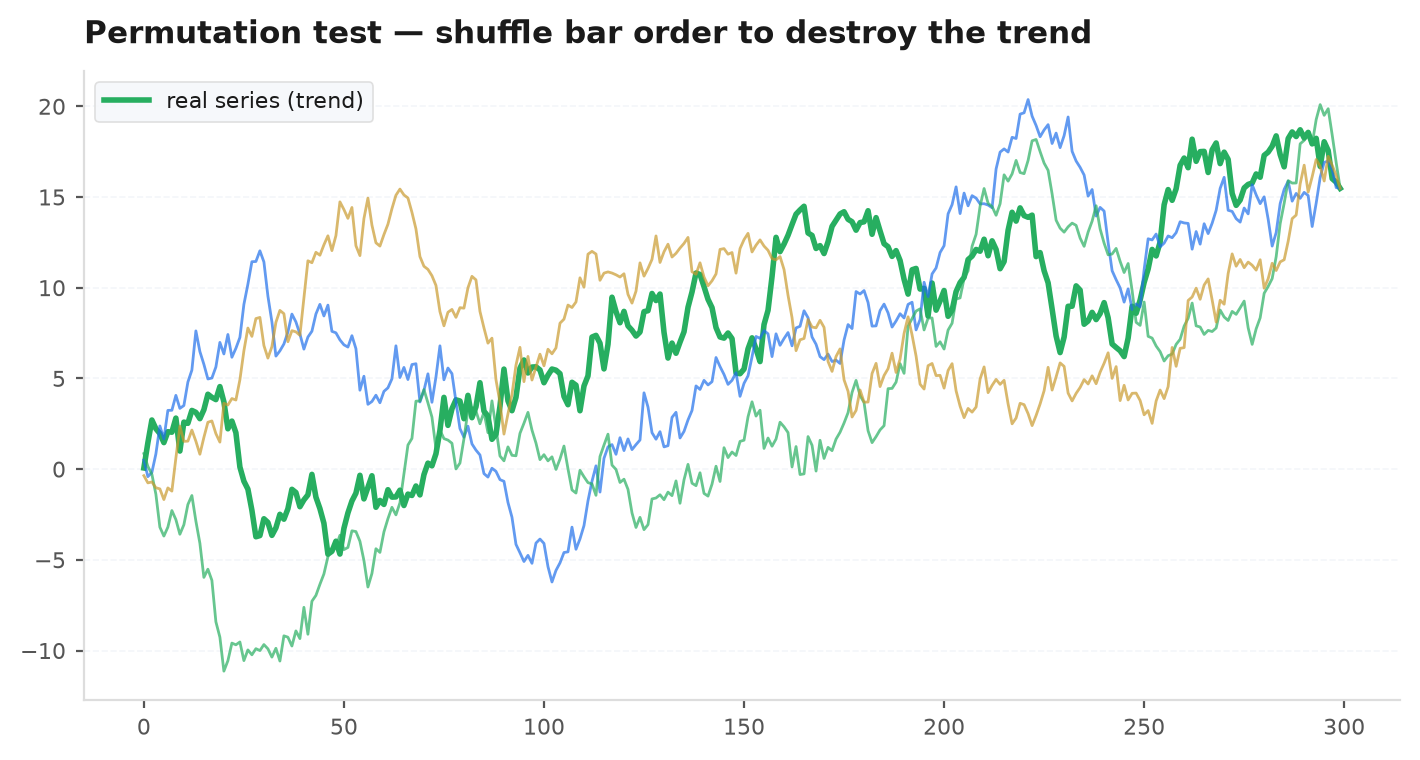
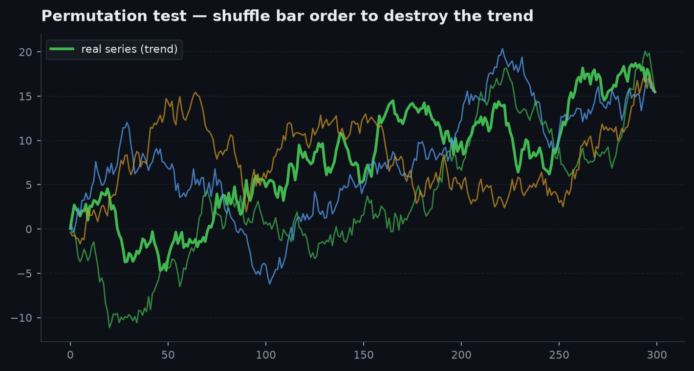
A trend or breakout strategy earns from the market's serial structure — the fact that moves persist. The permutation test builds a null world where that structure is gone but everything else is identical. Take the market, shuffle the order of its increments to erase trends and autocorrelation, but keep the exact set of returns. Re-run the strategy on this structure-free market and you have one sample of what it would earn on pure noise. Do it thousands of times and you have the whole null distribution.

A real trending price path beside a permuted path with identical returns but no trend — Left: the real path, with trends. Right: a permutation — same return marginal, structure destroyed. The strategy's earnings on the right are its null.

permute_ohlc — the correct null for bar strategies#

For anything that reads bars (breakouts, channels, candles), edgekit uses the Masters / NeuroTrader OHLC bar-permutation. It decomposes each log bar into four increments — the gap, high−open, low−open, close−open — applies one shared permutation to all four (so every rebuilt bar stays internally valid, with high ≥ open/close/low), then cumsums back into prices. The close-to-close return marginal is preserved exactly; the order is gone. Bar 0 is the untouched anchor.

permute_ohlc.py

def permute_ohlc(o, h, l, c, rng):
    lo, lh, ll, lc = np.log(o), np.log(h), np.log(l), np.log(c)
    n = len(c)
    pg = lo[1:] - lc[:-1]     # gap:   open - prev close
    ph = lh[1:] - lo[1:]      # high - open
    pl = ll[1:] - lo[1:]      # low  - open
    pc = lc[1:] - lo[1:]      # close - open
    j = rng.permutation(n - 1)
    pg, ph, pl, pc = pg[j], ph[j], pl[j], pc[j]   # SAME perm -> shape-consistent bars
    ...                                            # cumsum back into valid OHLC prices

!Match the null to the mechanism

Use permute_ohlc when the strategy reads bars; use permute_returns (a plain reshuffle of a return series) when it acts on returns directly. A mismatched null can leak the very structure you are trying to destroy — and a leaky null makes a fake edge look real.

The p-value#

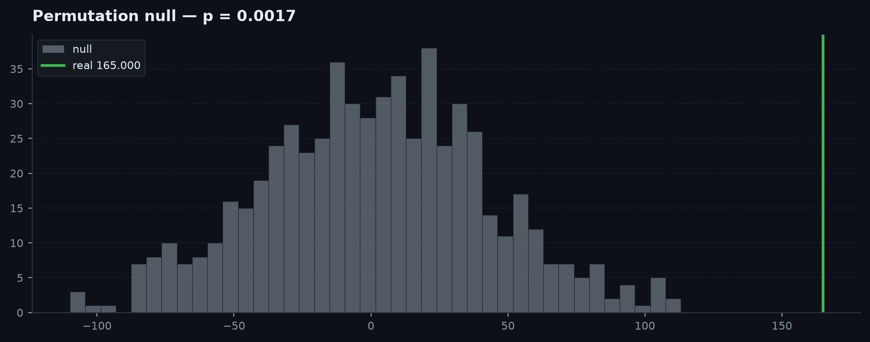
Let $s$ be your real statistic (total R, profit factor, whatever you chose) and $s_{1}^{*}, \dots, s_{N}^{*}$ the statistics on $N$ permuted markets. The Monte-Carlo permutation p-value is the fraction of null draws that matched or beat the real result:

p = \frac{1 + # { i : s _{i}^{*} \geq s }}{N + 1}

The $+ 1$ in both numerator and denominator is not cosmetic — it counts the observed sample as one of its own permutations, so the p-value can never be exactly zero. You have not proven impossibility from a finite sample, and the test stays valid. The floor is $1/ (N + 1)$ , so more permutations buy a tighter floor.

Decision rule: $p < 0.01$ means the edge is real — random data essentially never matched it. And the test's validity runs the other way too: a no-edge strategy (a breakout on a pure random walk) yields $p \sim U (0, 1)$ averaged over seeds — it is notspuriously significant. A test that only ever said "real" would be useless; this one correctly says "noise" when it is noise.

mcpt.py

import edgekit as ek
from edgekit.core import bootstrap_rng

real = strategy_total_r(bars)              # the real statistic

def null_fn(rng):
    po, ph, pl, pc = ek.validation.permute_ohlc(
        bars.open, bars.high, bars.low, bars.close, rng)
    return strategy_total_r(rebuild(po, ph, pl, pc))   # re-run on a shuffled market

p = ek.validation.mcpt(real, null_fn, n=1000, rng=bootstrap_rng())
print(f"permutation p = {p:.4f}")          # p < 0.01 -> real edge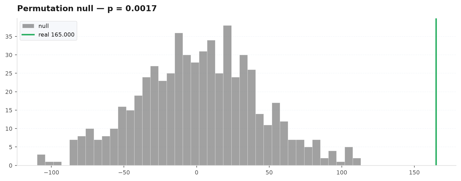

Histogram of the null statistic with the real result marked far in the right tail — The null distribution of the statistic under permuted markets. The real result (vertical marker) sits in the right tail — a small p-value.

A permutation test, worked end to end#

Let us run the whole thing on one concrete result so it stops being abstract. You have a Donchian breakout on BTCUSDT H4, and over the full sample it earned a total of +64R. That is your $s$ . The question is not "is +64R a lot?" — it is "could a market with no exploitable trends have handed the same strategy +64R by luck?" Here is exactly what happens, step by step:

Step 1 — pin the real number. Run the strategy once on the true BTCUSDT bars: $s = + 64$ R. Nothing shuffled yet.
Step 2 — build one null world. Call permute_ohlcwith a fresh RNG. It keeps every bar's gap/high/low/close increments but reorders them with one shared permutation, so the exact set of returns is preserved while the trends are destroyed. Rebuild that into a valid OHLC frame — a BTCUSDT that never was, with the same volatility and fat tails but no persistence.
Step 3 — re-run the strategy on it. Same Donchian rules, same cost, on the scrambled market. Say it earns $s_{1}^{*} = + 11$ R. That is one draw of "what this strategy makes on structure-free noise."
Step 4 — do it 1,000 times. Steps 2–3 with 1,000 different shuffles give a whole distribution $s_{1}^{*}, \dots, s_{1000}^{*}$ — mostly scattered around zero, a few lucky ones reaching +20R or +30R, because even noise occasionally lines up into a fake trend.
Step 5 — count and divide. Ask how many of the 1,000 null worlds matched or beat the real +64R. Suppose 4 did. Then $p = (1 + 4) / (1 + 1000) = 5/1001 \approx 0.005$ .

Read that verdict: on structure-free markets the strategy essentially never reaches +64R, so the trends it traded were real, not an accident of the return distribution. $p \approx 0.005 < 0.01$ — it clears the decisive gate. Now the counter-example, so you trust the test in both directions: run the same procedure on an SMA-cross whose true edge is zero and it earned +9R. This time roughly 380 of the 1,000 shuffles match or beat +9R, so $p = (1 + 380) / (1 + 1000) \approx 0.38$ . More than a third of pure noise did as well or better — the +9R is indistinguishable from luck, and you kill it. Same machine, opposite conclusion; that is what makes the p-value trustworthy rather than a rubber stamp.

✦At the desk — what a small p does and does not buy you

p \approx 0.005

says the structure is real; it says nothing about whether the edge is big enough to trade after cost, whether it survives the next regime, or whether you overfit the entry rule. It clears exactly one charge. That is why permutation is step 3 of the gauntlet, not the whole gauntlet — the ORB in the previous chapter clears permutation and still gets rejected at the cost gate.

Trade-order shuffling#

A related, cheaper permutation acts on the trade sequence rather than the market. Once you have a stream of per-trade R-multiples, their order was one accident of history. Shuffling that order many times and recomputing the equity curve shows how much of your drawdown and terminal wealth is down to sequence luck. It does not test whether the edge is real (the R-multiples are held fixed), but it does bound the path-dependent risk — the same idea as the block bootstrap, applied at the trade level.

Forward path simulation and confidence cones#

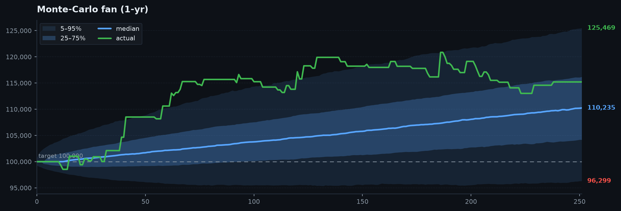
The bootstrap also runs forward. Resample blocks of daily returns into thousands of $H$ -day future paths and you get a distribution of equity curves. Plot their percentiles through time and you have a confidence cone (a fan chart): the median path down the middle, the 5th–95th percentile band widening as uncertainty compounds with the horizon.

fan.py

import edgekit as ek

mc = ek.validation.block_bootstrap_mc(daily_r, block=5, horizon=252, n=20000)
# mc["terminal"]  -> array of terminal cum-returns (one per path)
# mc["drawdowns"] -> array of per-path max drawdowns
# percentiles of the paths through time draw the confidence cone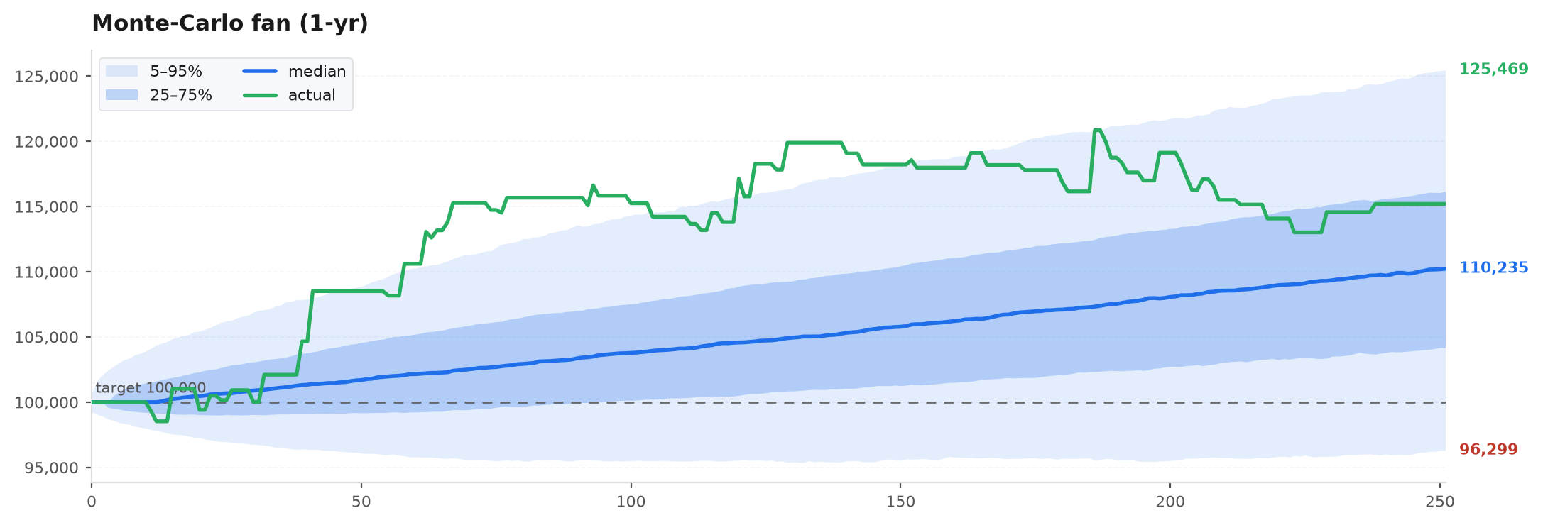

Fan chart of thousands of simulated forward equity paths with a widening percentile band — A confidence cone: the median forward path with a widening 5th–95th percentile band. Uncertainty compounds with the horizon.

Reading a fan chart#

The cone is a humility device. Two readings matter most: the width at your horizon (how uncertain the outcome is) and the lower edge (the bad-but-plausible case you must be able to survive). A fan whose 5th percentile dips deeply negative is telling you the strategy can lose money over a full year even if its expectancy is positive — plan capital and psychology around that lower band, never the median.

Risk of ruin via simulation#

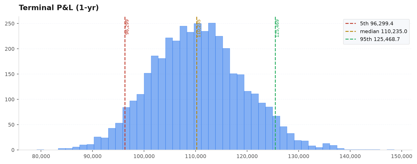
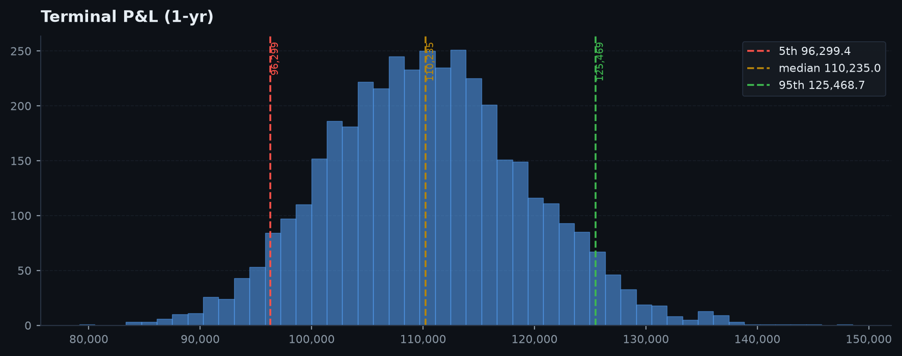
The terminal-wealth distribution answers the survival question directly. Risk of ruin is the fraction of simulated paths that breach a floor — a prop-firm drawdown limit, a personal stop-trading threshold — at any point along the path:

P_{ruin} = \frac{1}{n} k = 1 \sum n 1 [t \leq H min V_{t}^{(k)} < V_{floor}]

Because the block bootstrap preserves losing streaks, this estimate is honest where a closed-form Gaussian formula would be dangerously optimistic. The drawdown distribution from block_bootstrap_mc feeds straight into it, and dd95 is the one-number version: size so that even a 95th-percentile bootstrapped drawdown stays within your budget.

Histogram of terminal wealth across simulated paths with a ruin threshold marked — Terminal-wealth distribution across paths. The mass to the left of the floor is the simulated risk of ruin.

Putting the whole toolkit together#

mc_workflow.py

import edgekit as ek
from edgekit.core import bootstrap_rng

# 1. Is the edge real? Permutation test on the market structure.
def null_fn(rng):
    po, ph, pl, pc = ek.validation.permute_ohlc(
        bars.open, bars.high, bars.low, bars.close, rng)
    return strategy_total_r(rebuild(po, ph, pl, pc))
p = ek.validation.mcpt(strategy_total_r(bars), null_fn, n=1000, rng=bootstrap_rng())

# 2. How bad can it get? Block-bootstrap drawdown distribution.
mc    = ek.validation.block_bootstrap_mc(daily_r, block=5, horizon=252, n=20000)
worst = ek.validation.dd95(daily_r, horizon=252)

# 3. Size against the bootstrapped worst case, not the lucky historical one.
sized = ek.sizing.size_to_dd(daily_r, dd_budget=0.095, account=100_000)
print(p, worst, sized["dollar_per_r"])

✦Distributions, not point estimates

The recurring theme: a backtest is one sample; Monte Carlo turns it into a distribution. Use the permutation test to decide whether the edge is real, and the block bootstrap to decide how much of it you can afford to risk. Never size against the single realised drawdown — it was lucky by definition, because you only got to see the one path that happened.

Next: Walk-forward analysis — the out-of-sample discipline that keeps you from tuning on the very data you then report.