Cointegration & pairs

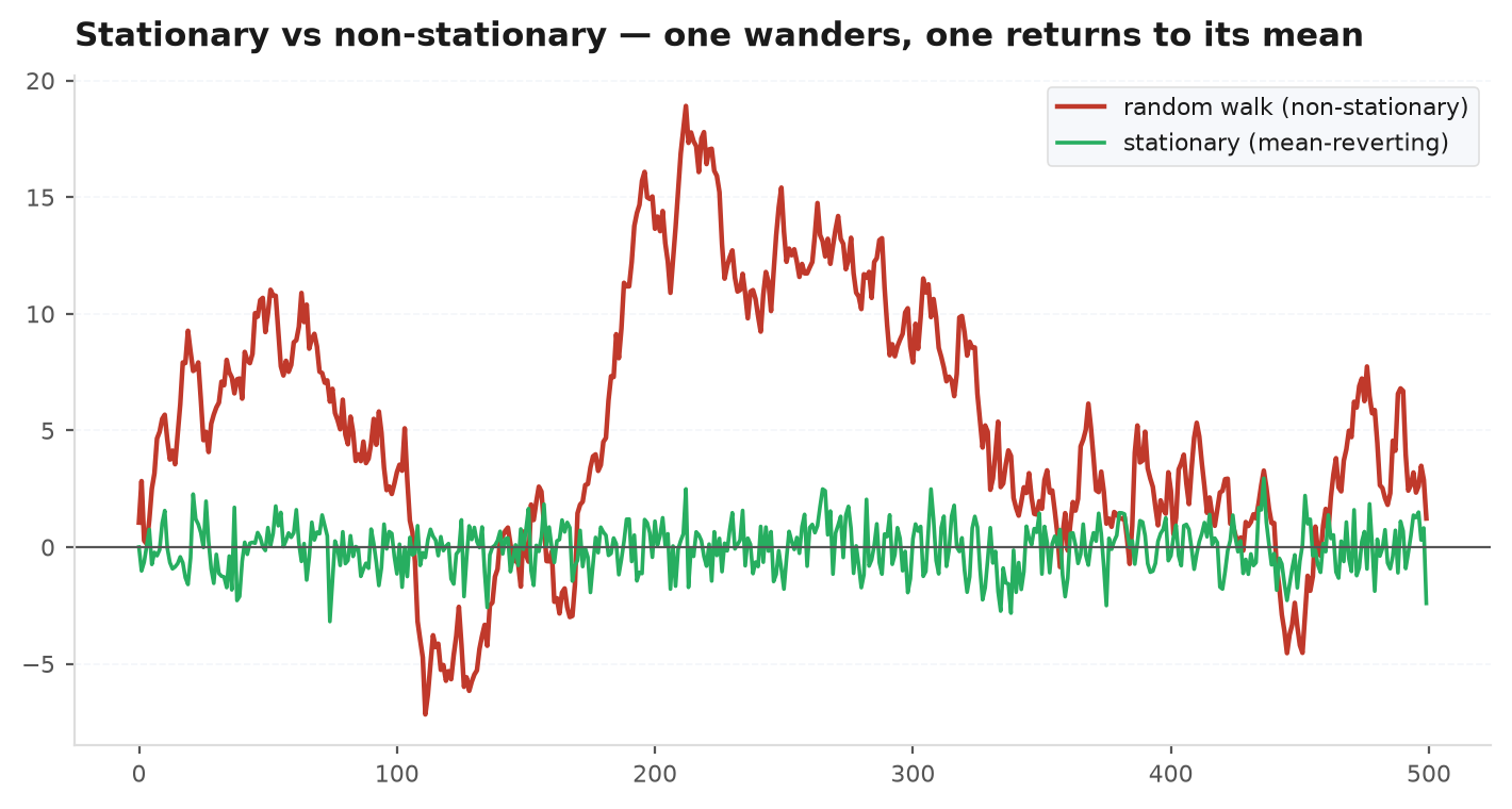
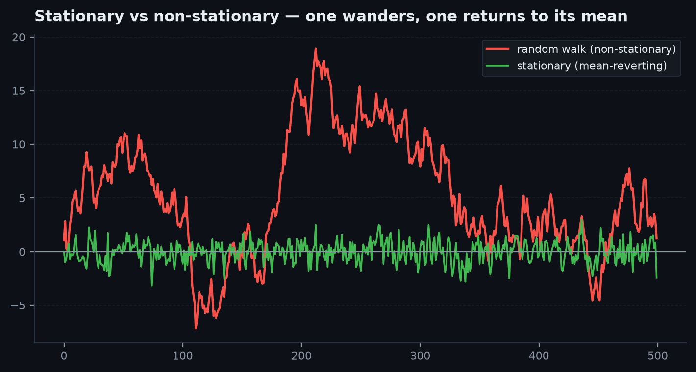
A single price is a random walk — non-stationary, no mean to trade against. But two prices can be individually non-stationary and yet tethered to each other, so that a particular combination of them is stationary. That combination is a spread, the tether is called cointegration, and the whole of market-neutral pairs trading is built on it: you cannot forecast where either leg goes, but you can bet the gap between them snaps back. This chapter is the mechanics — spotting a real relationship versus a fake one, estimating the hedge ratio, testing the spread, and modelling its mean-reversion.

✕This mechanism is real; most instances are not

Cointegration is a genuine, tradeable phenomenon — and also the single most over-claimed edge in retail quant. Two series can look beautifully co-moving over a window and be an artefact of a shared regime that then breaks. Everything below is necessary but not sufficient: a passing ADF stat is a reason to test properly, not a reason to trade. Take every candidate through permutation and out-of-sample checks in the gauntlet before it touches capital.

✦Why a trader cares

Coca-Cola and PepsiCo are the same business facing the same shocks — sugar prices, consumer spending, the dollar. Neither price is forecastable on its own (both are random walks), but when Coke runs up 4% and Pepsi does not, something has to give: history says the gap tends to snap back. You cannot bet on either stock, but you can bet on the spread between them closing — a trade that makes money whether the market goes up or down, because you are long one and short the other. This chapter is how you tell a real tether from a coincidence, size the hedge, and time the fade.

Spurious regression vs cointegration#

Regress one random walk on an unrelated second random walk and you will very often get a large $R^{2}$ and a t-statistic that screams significance. This is the spurious regression trap (Granger and Newbold, 1974): two independent I(1) series drift, and over any finite sample their drifts happen to line up enough to fool ordinary least squares. The regression is statistically meaningless — its residual is itself a random walk, so nothing pins the two series together.

Cointegration is the real thing that spurious regression imitates. Two series $y_{t}$ and $x_{t}$ are cointegrated if each is individually I(1) (a random walk in levels) but some linear combination is I(0) (stationary):

s_{t} = y_{t} - β x_{t} is stationary, y_{t}, x_{t} \sim I (1)

The economic picture is an equilibrium with a rubber band. Both prices wander freely, but whenever the spread $s_{t}$ stretches away from its mean, arbitrage-like forces pull it back. The distinction from spurious regression is entirely in the residual: for a spurious pair the residual is a random walk (ADF fails to reject); for a cointegrated pair the residual is stationary (ADF rejects). That test on the residual is the whole game.

A stationary mean-reverting spread beside a non-stationary random-walk residual — Top: the residual of a genuinely cointegrated pair oscillates around a fixed mean — stationary, tradeable. Bottom: the residual of a spurious pair wanders with no anchor — a random walk that only looked co-moving in-sample. The ADF test on the residual is what tells them apart.

The hedge ratio: static vs dynamic#

The spread only makes sense once you have a hedge ratio $β$ — the number of units of $x$ that neutralise one unit of $y$ . There are two ways to get it, and the choice matters.

Static: rolling OLS#

The Engle-Granger first step is an ordinary regression of one leg on the other, whose slope is the hedge ratio. A single full-sample OLS bakes in look-ahead (it uses the whole history to price today), so in practice you run it on a trailing window and let $β$ evolve. edgekit's rolling_ols_hedge returns the rolling intercept, slope, and residual in one call:

import edgekit as ek

# y, x are aligned price series (e.g. two related instruments' closes)
alpha, beta, resid = ek.indicators.rolling_ols_hedge(y, x, win=90)
# alpha[t], beta[t] use only the trailing 90 bars up to t  -> causal, no look-ahead
# resid[t] = y[t] - (alpha[t] + beta[t]*x[t])  is the spread

Rolling OLS is transparent and cheap, but it has a lag: the window must fill with new data before $β$ adapts, and a short window is jumpy while a long one is stale.

Dynamic: the Kalman filter#

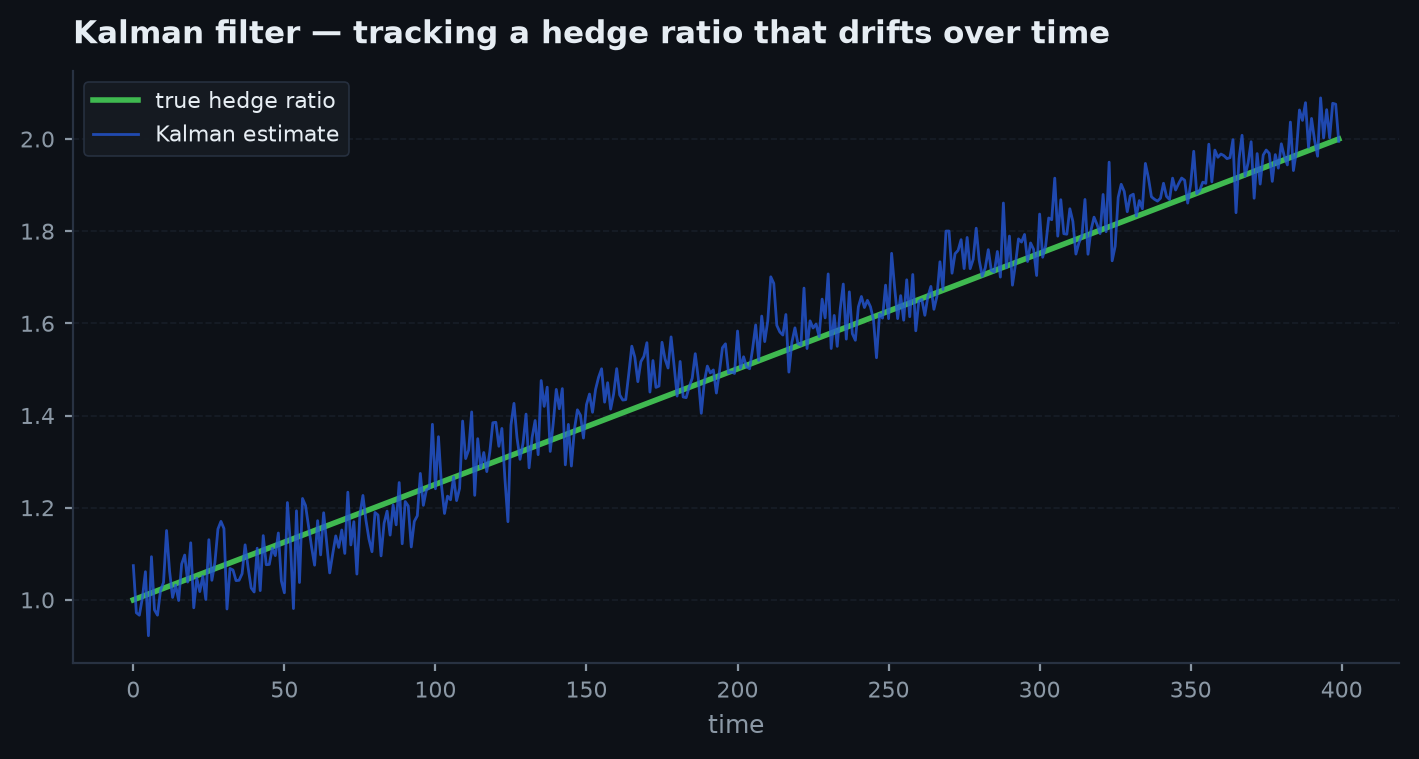
The Kalman filter treats the hedge ratio as a hidden state that drifts continuously, updating it every bar from the latest observation rather than re-fitting a window. It models $β_{t}$ as a random walk and $y_{t}$ as a noisy linear readout of it:

β_{t} = β_{t - 1} + w_{t}, y_{t} = α_{t} + β_{t} x_{t} + v_{t}

Two knobs govern its behaviour. $δ$ sets how fast the hedge ratio is allowed to wander (the state-transition variance) — larger $δ$ means a more adaptive, more nervous $β$ ; $r$ is the observation-noise variance. The filter's one-step prediction error is the spread, delivered causally with no window lag:

k = ek.timeseries.kalman_hedge(y, x, delta=1e-4, r=1.0)
# k == {"beta": ndarray,     # the dynamic hedge ratio, updated every bar
#       "alpha": ndarray,    # the dynamic intercept
#       "spread": ndarray}   # y - (alpha + beta*x), the tradeable series

spread = k["spread"]
hedge_now = k["beta"][-1]    # units of x to short per unit of y, right now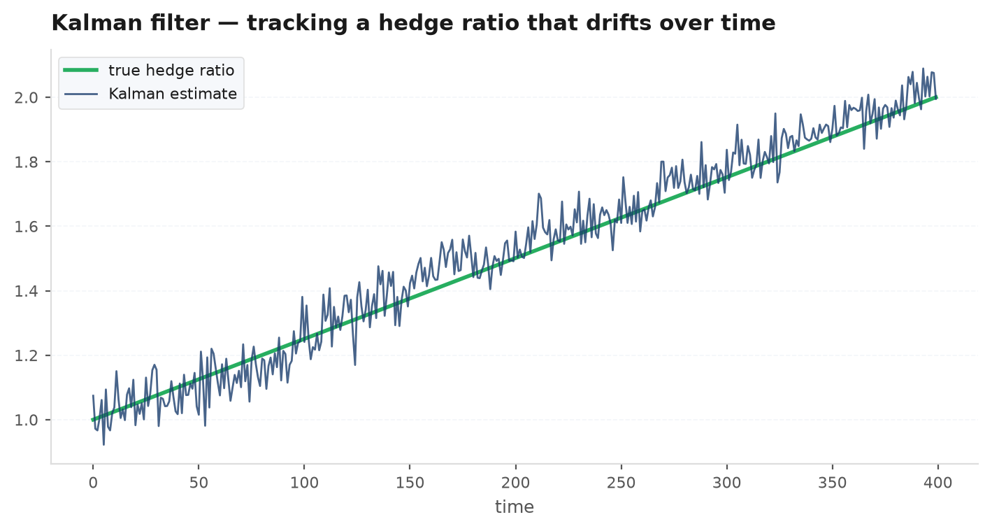

A dynamic Kalman hedge ratio adapting over time with the resulting spread below — Top: the Kalman-filtered hedge ratio beta_t evolves bar by bar as the relationship between the two legs drifts, with no fixed-window lag. Bottom: the resulting spread — the filter's prediction error — oscillates around zero, ready to standardise into a z-score.

✦Scenario: a hedge ratio that drifts from 1.0 to 1.5

Two gold miners, GOLDCO and MINEX, start the year moving one-for-one:

β \approx 1.0

, so you short one MINEX for every GOLDCO you buy. Over the year MINEX takes on leverage and its stock becomes roughly 50% more sensitive to the gold price than GOLDCO's. A static full-sample OLS would average the whole year and hand you a stale

β \approx 1.25

— wrong at both ends. A 90-day rolling OLS chases it, but always ~45 bars late. The Kalman filter, watching each bar's prediction error, walks

β_{t}

smoothly from

1.0 \to 1.5

as the drift happens, so today's hedge is

k ["beta"] [- 1] \approx 1.5

: you now short 1.5 MINEX per GOLDCO. Get this wrong and your “market-neutral” spread quietly picks up a directional gold bet — the drift is not a detail, it is the difference between neutral and naked.

✦Which to use

Rolling OLS is the honest baseline and easiest to reason about; reach for it first. The Kalman filter earns its keep when the true hedge ratio genuinely drifts (different volatilities, evolving lead-lag) and a fixed window is always either too slow or too jumpy. Whichever you use, the hedge ratio must be computed from past data only — both edgekit calls are causal by construction.

Engle-Granger: the two-step test#

The Engle-Granger procedure is the standard way to certify a pair, and it is exactly two steps:

Step 1 — estimate the spread. Regress $y$ on $x$ to get $β$ , then form $s_{t} = y_{t} - β x_{t}$ (via rolling_ols_hedge or kalman_hedge above).
Step 2 — test the residual for a unit root. Run the Augmented Dickey-Fuller test on the spread. If the spread is stationary (ADF rejects the unit root), the pair is cointegrated.

Recall from the time-series chapter that adf_stat returns the raw t-statistic, not a p-value — compare it to the critical values (below roughly $- 2.86$ is 5% significance, $- 3.43$ is 1%). The more negative, the more convincingly the spread reverts.

# Step 1: spread from the dynamic hedge (or use the rolling-OLS resid)
spread = ek.timeseries.kalman_hedge(y, x, delta=1e-4, r=1.0)["spread"]

# Step 2: ADF on the spread. More negative = more clearly mean-reverting.
t = ek.timeseries.adf_stat(spread, lags=1)
if t < -2.86:
    print(f"spread stationary at ~5% (adf t = {t:.2f}) -> candidate cointegrated pair")
else:
    print(f"cannot reject unit root (adf t = {t:.2f}) -> likely spurious, do not trade")

!The critical values are stricter here

Because the spread is itself an estimated residual (you fitted beta to it), the honest critical values are more negative than the textbook ADF ones — fitting the hedge ratio mechanically makes the residual look more stationary than it is. When a pair only barely clears

- 2.86

, treat it as a fail, not a pass.

✦Scenario: two ADF verdicts

Run adf_stat on the Coke-Pepsi spread over five years and it returns

t = - 3.6

— comfortably past the 1% critical value of

- 3.43

, so the spread convincingly reverts: a real candidate. Now run it on a spurious pair — say Coke against an unrelated oil driller that merely happened to trend together during a bull market — and you get

t = - 1.4

, nowhere near

- 2.86

: the residual is itself a random walk, no tether, do not trade it. Same code, same threshold, opposite decisions — and note that because you fitted the hedge ratio, a marginal

- 2.9

should still be read as a fail, not a pass.

The Ornstein-Uhlenbeck model of the spread#

A stationary spread is tradeable, but you want more than a yes/no — you want to know how fast it reverts and where it reverts to. The continuous-time model of exactly this is the Ornstein-Uhlenbeck process, the mean-reverting cousin of Brownian motion:

d s_{t} = κ (θ - s_{t}) d t + σ d W_{t}

Three parameters carry all the meaning. $θ$ is the equilibrium level the spread is pulled toward. $κ$ is the speed of that pull — larger $κ$ means faster reversion. $σ$ is the size of the random shocks fighting the pull. edgekit fits it by OLS on the AR(1) increments and hands back the derived half-life — the expected number of bars to close half the gap to equilibrium:

t_{1/2} = \frac{ln 2}{κ}

ou = ek.timeseries.ou_params(spread)
# ou == {"kappa": reversion speed,
#        "theta": equilibrium level,
#        "sigma": per-bar shock std,
#        "half_life": ln(2)/kappa bars}

# a convenience half-life is also on indicators:
hl = ek.indicators.half_life(spread)
print(f"kappa={ou['kappa']:.4f}  theta={ou['theta']:.4f}  half-life={ou['half_life']:.1f} bars")

The half-life is the most operationally useful number in the whole chapter: it is your holding horizon. A half-life of 5 bars says positions close in days and the pair can be traded actively; a half-life of 200 bars says you would hold for the better part of a year, tying up capital and exposing you to the relationship breaking before it reverts. A negative or huge $κ$ means no usable reversion — skip it.

✦Scenario: what the half-life tells you to do

ou_params on the Coke-Pepsi spread returns

κ \approx 0.069

, giving a half-life of

ln 2/0.069 \approx 10

trading days. Read operationally: when the spread gaps out, expect it to close half the gap in about two weeks — so this is a swing pair, not a day trade, and a position that has sat open for ~30 days (three half-lives) without reverting is a red flag that the tether may have snapped. Contrast a pair with

κ \approx 0.003

(half-life ≈ 230 days): you would tie up capital for the better part of a year per round-trip and take only a handful of independent bets — statistically too thin to trust however pretty the backtest. The half-life sets your holding horizon, your time-stop, and your realistic trade count all at once.

Trading the z-score#

With a stationary spread and a sane half-life, the trade rule writes itself: standardise the spread into a z-score and fade the extremes back toward $θ$ .

z_{t} = \frac{s _{t} - μ _{t}}{σ _{t}}

where $μ_{t}$ and $σ_{t}$ are a trailing mean and standard deviation of the spread (or the OU $θ$ and the stationary std). The canonical rule: short the spread (sell $y$ , buy $β$ of $x$ ) when $z_{t} > + 2$ , long the spread when $z_{t} < - 2$ , and flatten as $z_{t}$ crosses back through 0. Because both legs are held, the position is dollar-neutral and — if the cointegration holds — largely immune to the direction of the underlying market. You can build this as a BaseStrategy subclass that trades a synthetic spread instrument, sizing the two legs by the current hedge ratio.

# z-score of the causal spread against a trailing window (past data only)
import numpy as np
win = 60
s = np.asarray(spread, float)
mu = np.array([s[max(0, t - win):t].mean() for t in range(1, len(s) + 1)])
sd = np.array([s[max(0, t - win):t].std()  for t in range(1, len(s) + 1)])
z = (s - mu) / np.where(sd == 0, np.nan, sd)

# entry/exit rule inside a BaseStrategy on the synthetic spread:
#   z > +2   -> short spread (sell y, buy beta*x)
#   z < -2   -> long  spread (buy  y, sell beta*x)
#   |z| < 0.5 -> flat ; also time-stop after ~3x the OU half-life

✦Scenario: a z-score round-trip

Coke jumps on an earnings beat while Pepsi lags, and the spread stretches to

z = + 2.3

. The rule fires: short the spread — sell $100k of Coke, buy

β \approx 1.1

times that, $110k, of Pepsi, so the position is dollar-neutral and indifferent to whether the whole sector rises or falls. Over the next ~10 days (the half-life) the gap closes and

z

drifts back through 0; you flatten and book the convergence. Had

z

instead kept climbing to +4 and stayed there past ~30 days, the time-stop would pull you out at a loss — the correct response to a tether that has broken, not a reason to add. Same machinery fires the mirror trade at

z < - 2

→Half-life sets the bands and the patience

Tie the entry band and the max holding time to the half-life. If the OU half-life is 10 bars, a position that has not reverted in ~30 bars is telling you the relationship may have broken — a time-stop is as important as the z-score exit. This is the same “the model can stop being true” humility that runs through the whole tutorial.

The risks that actually kill pairs trades#

Cointegration breaks. The relationship is an empirical regularity, not a law. A merger, a balance-sheet shock, an index reconstitution, or a regime change can sever the tether permanently — and the spread you were fading simply trends away and never comes back. This is the dominant risk.
It was never real. A spurious pair that cleared a too-lenient ADF threshold in one window. The defence is the gauntlet: permutation-test the spread, split it out-of-sample, and confirm the ADF stat holds on data the hedge ratio was never fitted to.
Costs on two legs. Every round-trip pays spread and commission twice, and reversion edges are thin. A pair that is profitable gross can be dead net — always run ek.costs.cost_stress at multiples of your assumed cost.
Too few trades. A long half-life yields a handful of round-trips per year, so a great-looking backtest can rest on a statistically meaningless number of independent bets. Count trades, not just returns.

Next: Regime detection — cointegration holds in some regimes and breaks in others, so the natural companion question is how to detect which regime you are in. We fit a two-state hidden Markov model to label calm-vs-volatile (or trending-vs-choppy) regimes and gate a strategy accordingly.