ARIMA & GARCH

The previous chapter told you which world a series lives in. This one gives you the classical models that put numbers on it. ARIMA is the workhorse for the conditional mean of a series — where the next value is expected to land — and GARCH is the workhorse for the conditional variance — how big the next move is likely to be. The punchline you should carry into every design: for tradeable assets, mean models of returns are usually weak, while variance models are reliably useful. Understanding why is the whole lesson.

✦Why a trader cares

Two questions sit under every position you hold: where is the next return likely to land, and how bigis the next move likely to be? A tempting hope is that yesterday's Bitcoin return tells you today's direction — buy the model and print money. This chapter shows why that hope is almost always empty (the direction is close to a coin flip) and why the other question pays: after a wild day, tomorrow is very likely wild too. You cannot forecast the sign of the move, but you can forecast its size — and that forecast is what sizes your position, sets your stop, and tells you when to stand down.

→Fit means on returns, fit variance on the same returns

ARIMA and GARCH both assume a stationary input, so you feed them log returns, not prices — the “I” (integration/differencing) in ARIMA is precisely what turns a non-stationary price into a stationary return before an ARMA mean model is fitted. Prices are I(1); their log returns are I(0).

AR, MA, ARMA, ARIMA: the mean model#

An ARIMA model describes today's value as a linear combination of its own past values and past forecast errors. It has three integer orders, written $ARIMA (p, d, q)$ : $p$ autoregressive terms, $d$ differences to reach stationarity, and $q$ moving-average terms. Build it up one piece at a time.

AR(p) — autoregression#

An autoregressive model regresses the series on its own recent history. The workhorse special case is AR(1): today is a constant plus a fraction of yesterday plus noise.

x_{t} = c + ϕ x_{t - 1} + ϵ_{t}, ϵ_{t} \sim iid (0, σ^{2})

The single coefficient $ϕ$ is the entire story. When $∣ ϕ ∣ < 1$ the process is stationary and mean-reverting: it is pulled back toward its long-run mean $μ = c / (1 - ϕ)$ , and a shock decays geometrically at rate $ϕ$ per step. When $ϕ = 1$ the constant vanishes into a unit root and you are back to a pure random walk — no mean to revert to, which is exactly the case the ADF test hunts for. When $ϕ > 1$ the process explodes. The general order- $p$ form simply stacks more lags:

x_{t} = c + i = 1 \sum p ϕ_{i} x_{t - i} + ϵ_{t}

✦Scenario: reading phi off a mean-reverting series

Fit AR(1) to a daily z-scored pairs spread and it comes back

ϕ = 0.90

. Read it directly: today the spread keeps 90% of yesterday's deviation from its mean, so a shock decays geometrically and its half-life is

ln (0.5) / ln (0.90) \approx 6.6

days — a stretched spread closes half its gap in about a week, which is exactly the holding horizon a pairs trade needs. Contrast the neighbours:

ϕ = 0.99

means a 69-day half-life (barely reverting — capital tied up for months), while

ϕ = 0.5

reverts in a single day (fast, but the edge per trade is tiny). And

ϕ = 1

is the wall: no mean, a pure random walk, nothing to trade. The one coefficient tells you whether — and how fast — there is anything to fade.

MA(q) — moving average of shocks#

A moving-average model makes today a blend of past forecast errors rather than past levels — it gives the series a short, finite memory of shocks that dies out completely after $q$ steps.

x_{t} = c + ϵ_{t} + j = 1 \sum q θ_{j} ϵ_{t - j}

ARMA(p,q) is just the two glued together — AR terms for persistent level-memory, MA terms for transient shock-memory — and ARIMA(p,d,q) wraps an ARMA around the $d$ -th difference of the raw series. For daily prices you almost always take $d = 1$ (one difference = returns), so an ARIMA on prices is an ARMA on returns.

Reading the order off ACF and PACF#

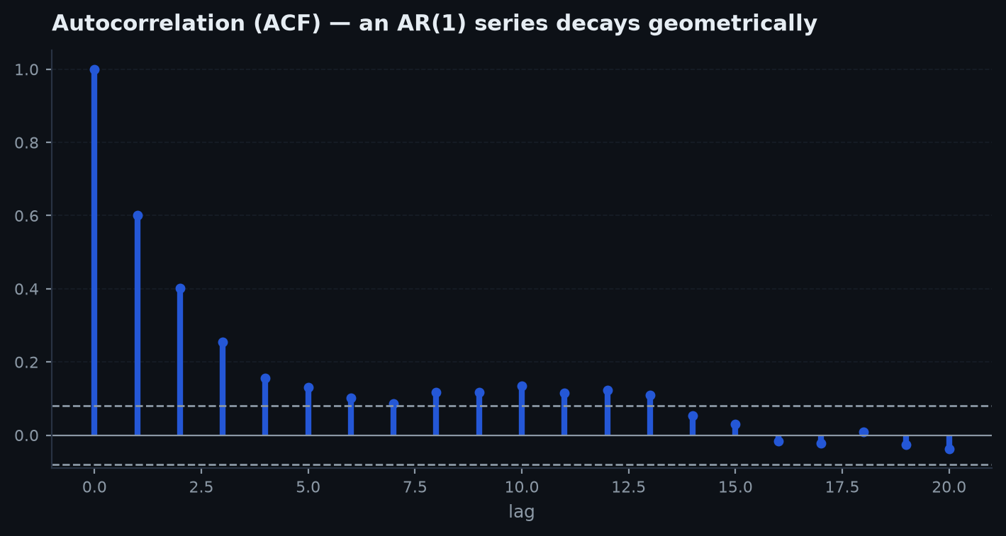
You do not guess $p$ and $q$ — you read them from the autocorrelation and partial-autocorrelation functions you met in the time-series chapter. The classic Box-Jenkins division of labour:

PACF cuts off after lag p, ACF decays gradually → an AR(p) process. The PACF isolates the direct effect of each lag once the shorter lags are partialled out, so an AR(p) shows exactly $p$ significant partial spikes then silence.
ACF cuts off after lag q, PACF decays gradually → an MA(q) process — the mirror image.
Both decay gradually → a mixed ARMA; pick the smallest orders that whiten the residuals.

edgekit gives you both functions directly (the PACF via the Durbin-Levinson recursion, no statsmodels), plus the white-noise band $\pm 1.96/ n$ to judge which spikes are real.

import edgekit as ek

rets = ek.timeseries.log_returns(bars.close)      # stationarise: prices -> returns

ac = ek.timeseries.acf(rets, nlags=40)            # ac[0] == 1 by construction
pc = ek.timeseries.pacf(rets, nlags=40)           # partial autocorrelations
band = 1.96 / len(rets) ** 0.5                    # +/- significance band

# how many PACF spikes poke outside the band -> candidate AR order p
p_hat = sum(1 for v in pc[1:11] if abs(v) > band)
print("suggested AR order:", p_hat)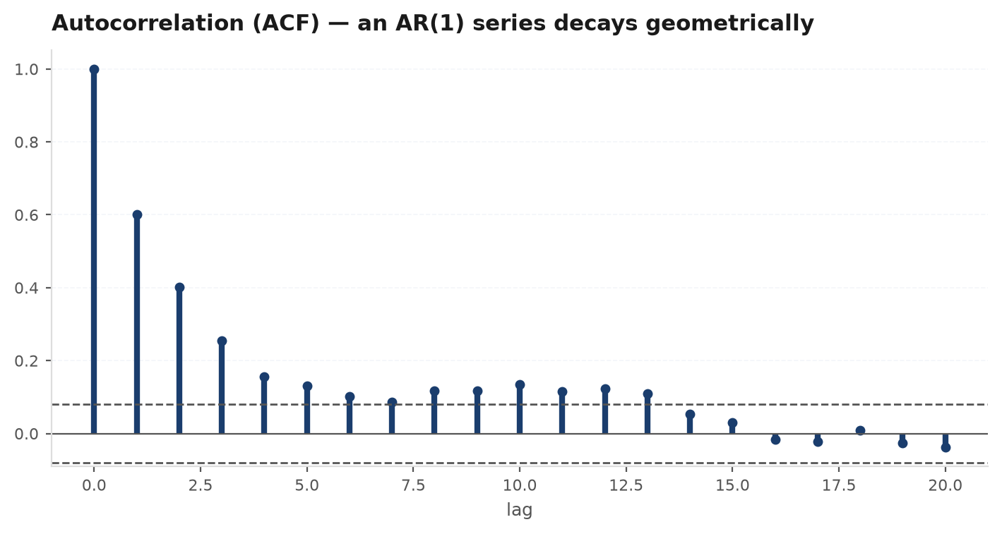

ACF and PACF of a return series with the significance band — ACF (top) and PACF (bottom) with the +/-1.96/sqrt(n) band shaded. For returns the bars typically sit inside the band at almost every lag — the fingerprint of near-white noise, and the reason a mean model of returns rarely pays.

!Why mean models of returns are weak

Run the ACF on returns and you usually find nothing significant past lag 0 — returns are close to serially uncorrelated. That is not a bug in the method; it is the near-efficiency of liquid markets. An ARIMA fit to such a series will have tiny coefficients, an

R^{2}

a hair above zero, and forecasts that collapse to the mean within a step or two. Fitting more lags just fits noise. This is the empirical wall behind the whole tutorial's insistence that directional edges are rare and must survive the gauntlet.

The twist: variance is predictable even when direction is not#

Here is the fact that redirects the entire modelling effort. Run the ACF on returns and it is flat. Run the same ACF on squared returns (a proxy for variance) and you find strong, slowly-decaying positive autocorrelation. Direction is unpredictable; magnitude is not. Big moves cluster with big moves, calm with calm — the volatility clusteringyou saw last chapter. Returns are, in the famous phrase, “serially uncorrelated but not independent.”

# direction: essentially no memory
lb_ret = ek.timeseries.ljung_box(rets, lags=10)        # small Q -> can't reject white noise

# magnitude: strong, persistent memory
lb_sq  = ek.timeseries.ljung_box(rets ** 2, lags=10)   # large Q -> squared returns ARE autocorrelated

✦Scenario: the same series, two verdicts

Run this on a few years of daily equity-index returns and the two Ljung-Box statistics come back worlds apart. On the returns,

Q \approx 8

across 10 lags — below the 5% critical value

χ_{10}^{2} = 18.3

, so you cannotreject “white noise”: the direction has no exploitable memory. On the squared returns of the identical series,

Q \approx 240

— off the chart, overwhelmingly significant. Same data, opposite answers: tomorrow's sign is a coin flip, but tomorrow's sizeis strongly predictable from today's. That single contrast is why the rest of this chapter models variance, not mean.

This asymmetry is why the profitable modelling target for most assets is variance, not mean. You may not know which way the next move goes, but you can forecast how big it will be — and that forecast is what sizes a position, sets a stop, and decides whether to be in the market at all.

GARCH(1,1): the variance model#

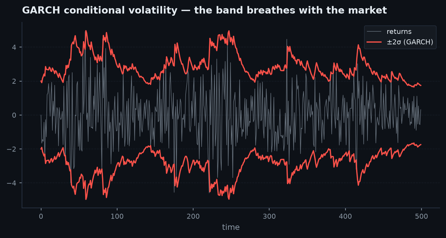
The ARCH/GARCH family models the conditional variance as its own recursion. The GARCH(1,1) — the version that wins in practice almost regardless of asset — says tomorrow's variance is a weighted blend of three things: a constant long-run level, yesterday's squared shock, and yesterday's variance.

σ_{t}^{2} = ω + α ϵ_{t - 1}^{2} + β σ_{t - 1}^{2}

Read each term. $ω > 0$ is the baseline variance the process relaxes toward. $α$ is the reaction: how sharply variance jumps in response to a fresh shock $ϵ_{t - 1}$ . $β$ is the memory: how much of yesterday's variance carries into today. Their sum is the single most important diagnostic:

persistence = α + β

Stationarity requires $α + β < 1$ ; the closer that sum sits to 1, the more slowly a volatility shock decays and the longer high-vol regimes persist. Typical equity and crypto fits land around $α \approx 0.05 - 0.15$ and $β \approx 0.8 - 0.9$ , i.e. persistence near $0.95$ — shocks fade over weeks, not days. The implied long-run (unconditional) variance is:

σ ˉ^{2} = \frac{ω}{1 - α - β}

edgekit fits the model by maximum likelihood using a derivative-free pattern search in pure numpy (no scipy), enforcing $ω > 0, α, β \geq 0, α + β < 1$ . It returns the parameters, the fitted conditional-volatility path, a one-step forecast, and the persistence:

g = ek.timeseries.garch11(rets, max_iter=200)
# g == {"omega", "alpha", "beta",
#       "cond_vol": ndarray of sigma_t,   # the fitted per-bar volatility path
#       "forecast": next-step sigma,      # sqrt(omega + alpha*r[-1]**2 + beta*sigma[-1]**2)
#       "persistence": alpha + beta}

print(f"alpha={g['alpha']:.3f}  beta={g['beta']:.3f}  persistence={g['persistence']:.3f}")
print("next-bar vol forecast:", g["forecast"])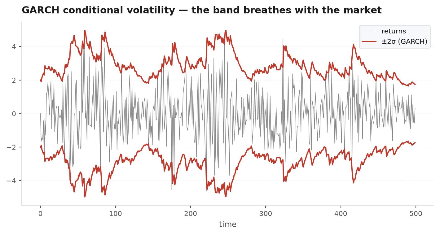

A return series with its GARCH(1,1) conditional volatility path overlaid — The GARCH(1,1) conditional volatility (line) tracks the return series (points): it ramps up as a cluster of large moves arrives and decays through the calm that follows, at a speed set by the persistence alpha+beta.

✦Scenario: a GARCH vol forecast the day after a Bitcoin crash

Fit GARCH(1,1) to daily Bitcoin returns and you get something like

α = 0.09, β = 0.88

(persistence

0.97

), with a long-run daily vol around 3.5%. Yesterday BTC was quietly running at

σ_{t - 1} = 3%

(variance 0.0009) — then it printed a

- 12%

day. Plug the shock into the recursion:

σ_{t}^{2} = ω + 0.09 (- 0.12)^{2} + 0.88 (0.03)^{2} \approx 0.0000368 + 0.001296 + 0.000792 = 0.00213

σ_{t} \approx 0.00213 = 4.6%

daily — an annualised jump from

\approx 57%

\approx 88%

(

\times 365

). The model just told you, quantitatively, that tomorrow's expected range is nearly double last week's. If your stop was a 2× multiple of forecast vol, it should widen accordingly; if you size to constant risk, your position should roughly halve. That is the forecast doing its one job.

Forecasting volatility forward#

The one-step forecast is mechanical — plug the latest shock and variance into the recursion. Multi-step forecasts mean-revert toward the long-run level $σ ˉ^{2}$ at rate $(α + β)$ per step:

E [σ_{t + h}^{2}] = σ ˉ^{2} + (α + β)^{h} (σ_{t + 1}^{2} - σ ˉ^{2})

With persistence near $0.95$ , the half-life of a vol shock is roughly $ln (0.5) / ln (0.95) \approx 13$ bars — so a spike today still meaningfully elevates your risk estimate a couple of weeks out. That horizon is the practical output: it tells you how long to keep stops wide and size trimmed after a shock.

✦GARCH vs EWMA

The RiskMetrics EWMA volatility from the last chapter is exactly a GARCH(1,1) with

ω = 0

and

α + β = 1

(a fixed

λ = β = 0.94

). EWMA is the cheap, zero-fit approximation; GARCH earns the extra

ω

term by adding genuine mean-reversion in variance, so its forecasts pull back to a long-run level instead of drifting. Use EWMA to size live and GARCH to understand and forecast.

What you actually do with this#

You will not usually trade an ARIMA point-forecast of returns — the ACF already warned you it is noise. What GARCH buys you is volatility-aware everything, and edgekit's strategy templates are built to consume it:

Volatility targeting. Feed the conditional-vol forecast into ek.sizing.vol_target so position size shrinks when GARCH says a storm is coming and grows in calm — keeping risk, not notional, constant.
Adaptive stops. A stop set as a multiple of forecast vol widens automatically in stress, so you are not shaken out by a normal move that merely looks large against a stale fixed distance.
Regime awareness. A persistence near 1 with an elevated current $σ_{t}$ is a quantitative “high-vol regime” flag — which is the exact idea the next-but-one chapter formalises with a hidden Markov model.

# GARCH-forecast vol -> size to a constant risk target, in a BaseStrategy subclass
g = ek.timeseries.garch11(rets, max_iter=200)
forecast_vol = g["forecast"]                       # next-bar sigma

# annualise for the sizing call (per-bar -> per-year), then target e.g. 15% vol
ann_vol = forecast_vol * (252 ** 0.5)
# vol_target scales an existing return/position stream toward the target vol path

✕A fitted model is a description, not a promise

GARCH parameters are estimated on one finite window and drift over time — persistence in a bull-quiet year differs from a crisis year. A vol forecast tells you the conditional risk given recent history; it says nothing about a discontinuous gap or a structural break. Treat the forecast as a live risk input to be stress- tested, never as a guarantee, and prove any strategy that leans on it through the full validation gauntlet.

Next: Cointegration & pairs — when two non-stationary prices move together closely enough that their spread is stationary, and how to estimate the hedge ratio, test the residual, and model the spread as a mean-reverting process you can actually trade.