Risk management

Every earlier chapter was about finding and sizing an edge. This one is about surviving long enough to collect it. Risk management is the discipline of quantifying how much you can lose — in a normal day, in a bad tail, and over a long ugly stretch — and then sizing so that the worst plausible outcome does not end the game. The measures here (VaR, Expected Shortfall, drawdown, the ulcer index) are the vocabulary; the sizing tools turn a risk target into a position. The through-line: a strategy with a real edge and reckless sizing is a losing strategy.

✦Why a trader cares

You are running a $100,000account. The single most important number in your life is not your expected return — it is the answer to “how much can I lose on a bad day, and how much on a truly awful one?” Guess too low and one tail event ends the account before the edge ever pays off; guess too high and you trade so small the edge is pointless. This chapter is the vocabulary for pinning that number down — VaR for the bad day, Expected Shortfall for the awful one, drawdown for the long ugly stretch — and then the sizing tools that turn a loss budget back into a position.

Position risk vs portfolio risk#

There are two distinct questions, and conflating them is a classic error. Position risk is how much a single trade can lose — governed by the entry, the stop, and the size, and expressed cleanly in edgekit as the R-multiple (loss at the stop = 1R). Portfolio risk is how much the whole book can lose at once, which is notthe sum of the position risks because positions are correlated. Two “independent” long trades that both crater in the same crash are, in that moment, one position twice the size.

The variance of a portfolio makes the correlation explicit. For weights $w$ and covariance matrix $Σ$ :

σ_{p}^{2} = w^{⊤} Σ w = i \sum w_{i}^{2} σ_{i}^{2} + i \neq = j \sum w_{i} w_{j} σ_{i} σ_{j} ρ_{ij}

The cross terms are the whole story of diversification: low or negative $ρ_{ij}$ shrinks portfolio risk below the sum of parts, while correlations that spike to 1 in a crisis (as they notoriously do) erase the diversification exactly when you need it. Manage risk at the portfolio level, not one trade at a time.

✦Scenario: the diversification that evaporates in a crash

Split the $100k book equally across two strategies, each running 12% annual volatility, normally correlated at

ρ = 0.2

. Portfolio vol is

0.0072 (1 + ρ) = 0.0072 \times 1.2 \approx 9.3%

— comfortably below either leg's 12%, the diversification working as advertised. Now a crisis hits and the two books, which looked independent in calm, both dump together:

ρ \to 0.9

. Portfolio vol jumps to

0.0072 \times 1.9 \approx 11.7%

— almost the full undiversified 12%. The benefit you sized against in calm nearly vanished in the exact moment you were counting on it. This is why the correlation-to-1 stress test at the end of the chapter is not optional.

Value-at-Risk#

Value-at-Risk answers: “over this horizon, what loss will I not exceed with confidence $1 - α$ ?” Formally it is the $α$ -quantile of the loss distribution — the 5% VaR is the loss such that only 5% of days are worse.

VaR_{α} = - in f {ℓ : P (R \leq ℓ) \geq α} = - Q_{R} (α)

edgekit reports VaR as a positive loss number (a 5% VaR of $0.03$ means “lose 3% or more on the worst 1-in-20 days”), with three estimation methods that trade off assumptions against tail realism:

Historical. The empirical $α$ -quantile of realised returns — no distributional assumption, but limited to tails your sample actually contains.
Gaussian. $- (μ + z_{α} σ)$ with $z_{α} = Φ^{- 1} (α)$ . Clean and cheap, but it assumes normality and so underestimates the tail for the fat-tailed returns you met in Part II.
Cornish-Fisher. The Gaussian quantile corrected for skewness and excess kurtosis, so a fat, left-skewed tail widens the VaR beyond the naive Gaussian estimate — a pragmatic middle ground.

import edgekit as ek

# rets: the strategy's daily return series (positive VaR = loss fraction)
var_hist = ek.risk.value_at_risk(rets, alpha=0.05, method="historical")
var_norm = ek.risk.value_at_risk(rets, alpha=0.05, method="gaussian")
var_cf   = ek.risk.value_at_risk(rets, alpha=0.05, method="cornish_fisher")
# fat/left-skewed tails -> var_cf > var_norm : the Gaussian number was too optimistic

✦Scenario: a 95% VaR on the $100k book, three ways

Your strategy's daily returns average roughly 0 with a 1% standard deviation, and they are fat-tailed and left-skewed (as real returns are). Compute the 5% (95%-confidence) 1-day VaR:
• Historical — the empirical 5th percentile of your actual daily returns comes in at

- 2.1%

, so

VaR = 2.1%

, i.e. $2,100on the $100k book. Read it as: “on the worst 1-day-in-20 I lose $2,100 or more.”
• Gaussian —

- (μ + z_{0.05} σ) = - (0 - 1.645 \times 0.01) = 1.6%

, or $1,645. Cleaner, but it assumes normality and so understates the loss by ~$450.
• Cornish-Fisher — correct the Gaussian quantile for the negative skew and fat tails and it widens to

\approx 2.4%

, or $2,400, now above the historical estimate because it extrapolates the tail shape rather than being capped by your sample.
Same book, same day: the ordering

Gaussian < historical < Cornish-Fisher

is the fat left tail making itself felt, and the Gaussian $1,645 is exactly the number that lulls accounts into over-sizing.

!The critiques of VaR

VaR has two deep flaws. First, it says nothing about how bad the tail is beyond the threshold — a 5% VaR of 3% is identical whether the worst 5% of days average −4% or −40%. Second, it is not a coherent risk measure: VaR can violate sub-additivity, meaning the VaR of a combined book can exceed the sum of its parts, which perversely penalises diversification. Both problems are exactly what Expected Shortfall fixes.

Expected Shortfall (CVaR)#

Expected Shortfall — equivalently Conditional VaR — answers the question VaR dodges: given that you are in the worst $α$ tail, what is the average loss? It is the mean of the tail, not its edge:

ES_{α} = - E [R ∣ R \leq Q_{R} (α)] \geq VaR_{α}

Because it averages over everything past the threshold, ES is always at least as large as VaR for the same $α$ , and it responds to the shape of the extreme tail. Crucially it is a coherent risk measure: it satisfies sub-additivity, so diversification can only reduce it — which is why regulators and serious risk desks size against ES, not VaR. edgekit gives you both in one pass, guaranteed internally consistent ( $cvar \geq var$ ):

tail = ek.risk.var_cvar(rets, alpha=0.05, method="historical")
# tail == {"var": positive loss, "cvar": positive loss >= var}
print(f"5% VaR = {tail['var']:.3%}   5% CVaR = {tail['cvar']:.3%}")

# the two standalone forms are also available:
es = ek.risk.expected_shortfall(rets, alpha=0.05, method="historical")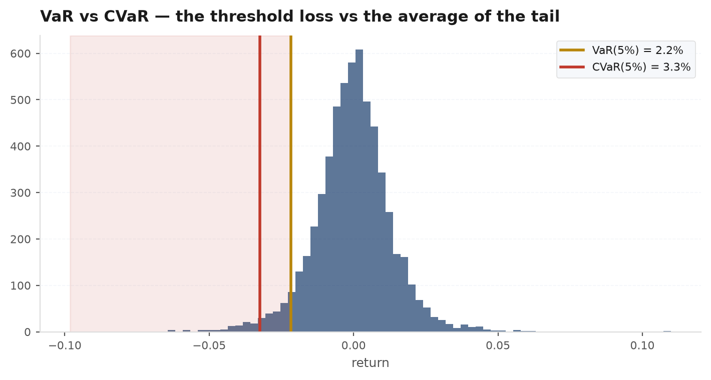

A return distribution with the VaR threshold and the CVaR tail mean marked — The return histogram with the 5% VaR marked as the quantile line and CVaR as the mean of the shaded tail beyond it. VaR is where the tail begins; CVaR is how deep it goes. For fat-tailed returns the gap between them is wide — and it is the gap that ruins accounts.

✦Scenario: what VaR did not tell you about the $100k book

The historical VaR said you lose at least $2,100 on the worst 1-in-20 days. But how bad are those days on average? Take the mean of every return past the 5th-percentile threshold and, for this fat-tailed book, it comes to

- 3.4%

— a 5% CVaR of $3,400. VaR told you where the tail begins ($2,100); CVaR tells you how deep it goes once you are in it ($3,400), a 60% larger number. That $3,400 — not the $2,100 — is what you must be financially and psychologically able to absorb, and it is why regulators and serious desks size against ES. The gap between the two is the fat tail, and it is the gap that empties accounts.

Tail risk and fat tails#

This all matters only because returns are not Gaussian. As Part II's distributions chapter showed, financial returns have excess kurtosis— fat tails — so “6-sigma” days that a normal model deems impossible show up every few years. The tail ratio is a quick, distribution-free read on the asymmetry: the size of the right tail relative to the left.

tail ratio = \frac{∣ Q _{R} ( 1 - q ) ∣}{∣ Q _{R} ( q ) ∣}, q = 0.05

A ratio above 1 means the winning tail is fatter than the losing tail (favourable convexity — small losses, occasional big wins, like a trend follower); below 1 flags crash-prone payoffs where you win small and lose big. Read it alongside CVaR to characterise the shape of what you are exposed to.

tr = ek.risk.tail_ratio(rets, q=0.05)   # |95th pctile| / |5th pctile|
# > 1 : right tail fatter (convex) | < 1 : left tail fatter (crash-prone)

Drawdown control and the ulcer index#

VaR and ES describe a single period. But what actually forces capitulation — and, on a prop account, breaches the drawdown limit — is the path: how far below its high-water mark the equity curve sits, and for how long. The drawdown series is the running loss from the prior peak, as a positive fraction:

D_{t} = \frac{max _{s \leq t} E _{s} - E _{t}}{max _{s \leq t} E _{s}}

Its maximum is the familiar max-drawdown, but a single scalar hides the difference between one sharp dip and a two-year slog underwater. The ulcer index captures that by taking the root-mean-square of the drawdown path — penalising drawdowns that are both deep and long, quadratically:

UI = \frac{1}{T} t = 1 \sum T D_{t}^{2}

# equity is the cumulative-return / account-value curve
dd = ek.risk.drawdown_series(equity)   # per-bar drawdown, 0 at every new high
ui = ek.risk.ulcer_index(equity)       # RMS of the drawdown path; deep+long hurts most
print(f"max drawdown = {dd.max():.2%}   ulcer index = {ui:.4f}")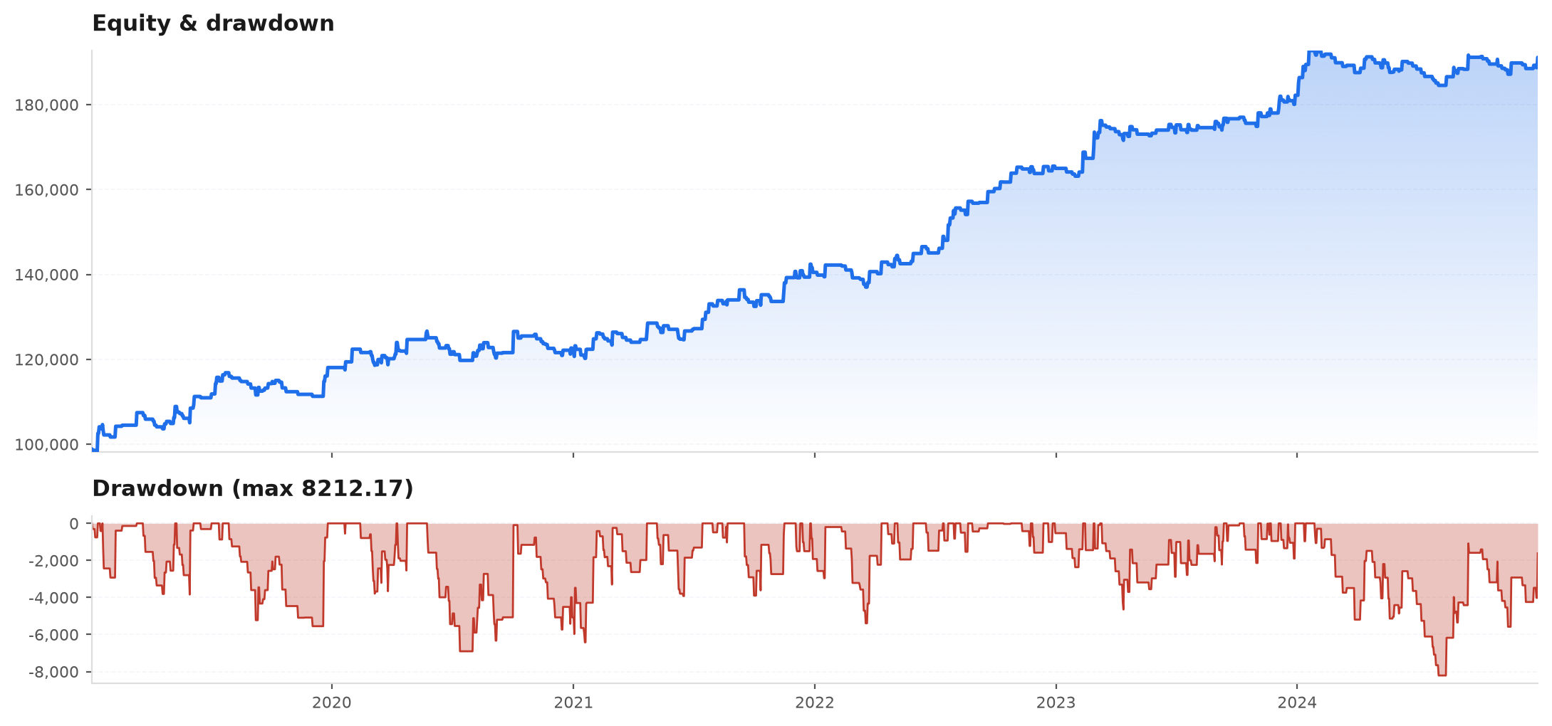

An equity curve with its underwater drawdown series plotted beneath — Top: the equity curve with its high-water mark. Bottom: the underwater plot — the drawdown series, zero at every new high and diving during losing stretches. The ulcer index is the RMS depth of that underwater region; two curves with the same max-DD can have very different ulcer indices.

✦Scenario: two curves, same max-drawdown, very different pain

Two strategies both post a 20% max-drawdown, so on that one number they look identical. Curve A took a sharp −20% hit and clawed back to new highs within a month — its underwater plot is a single deep spike, and its ulcer index is small (say

\approx 0.04

). Curve B drifted −20% down and then languished underwater for two years before recovering — a long shallow bathtub, ulcer index

\approx 0.12

, three times A's. Max-drawdown cannot tell them apart; the ulcer index, which RMS-averages the whole underwater path, says B was three times as painful to hold. If you have ever abandoned a “working” strategy out of sheer fatigue, it was the ulcer index, not the max-DD, that broke you.

✦Ulcer index over max-drawdown for comparing curves

Max-drawdown is a single worst-case point and is noisy — it can be set by one bar. The ulcer index integrates the entire pain of the curve, so it is the more stable statistic for ranking strategies and the better denominator for a pain-adjusted return (the Martin ratio = CAGR / ulcer index).

Risk budgeting: equal risk contribution#

At the portfolio level, the naive move is to allocate capital equally. The better move is to allocate risk equally — because a volatile asset given equal capital dominates the portfolio's variance. Equal risk contribution (risk parity) chooses weights so that each asset contributes the same amount to total portfolio risk. Asset $i$ 's marginal contribution is:

RC_{i} = w_{i} \frac{( Σ w ) _{i}}{w ^{⊤} Σ w}, ERC: RC_{i} = RC_{j} \forall i, j

There is no closed form, so ek.optimize.equal_risk_contribution solves it iteratively from the covariance matrix, and ek.sizing.risk_parity applies the rolling-volatility version bar by bar to a matrix of return streams:

import numpy as np

# covariance of the books' return streams -> equal-risk-contribution weights
cov = np.cov(np.vstack([book_a, book_b, book_c]))
w = ek.optimize.equal_risk_contribution(cov, iters=200)
# each book now contributes equally to portfolio variance -> no single book dominates

# or size a live book of streams to rolling risk parity:
weights = ek.sizing.risk_parity(returns_matrix, win=90)

✦Scenario: equal capital vs equal risk across three books

You allocate the $100k across three strategies: a trend follower at 20% vol, a pairs book at 8% vol, and a breakout at 12% vol, roughly uncorrelated. Split capitalequally (⅓ each) and the trend follower — with more than double the pairs book's volatility — ends up producing over half the portfolio's risk: one book quietly runs the show. Feed the covariance to equal_risk_contribution and it rebalances toward the inverse-volatility mix — roughly 19% to the trend book, 48% to the calm pairs book, 32% to the breakout — so each contributes the same one-third of portfolio variance. Same three edges, but now no single book can sink the account on its own bad month.

Sizing to a risk target#

Risk measurement is only useful if it feeds back into position size. Two edgekit sizers close that loop. vol_target scales exposure so realised volatility tracks a target — lever up in calm, cut in stress — which is the operational form of the GARCH-forecast idea from the first chapter of this part:

scale_{t} = min (\frac{σ _{target}}{σ ^ _{t}}, cap)

# vol-target an existing return/position stream (capped leverage)
scaled = ek.sizing.vol_target(port_returns, cap=1.5, win=60)

size_to_dd goes the other way: it sizes to a drawdown budget — the maximum you are willing to lose from peak — which is exactly the constraint a prop-firm challenge imposes. Give it the return stream, the drawdown budget, and the account size, and it backs out the position scale consistent with that limit:

# size so the expected peak-to-trough loss respects a fixed drawdown budget
size = ek.sizing.size_to_dd(daily_r, dd_budget=0.10, account=100_000)
# e.g. "never risk more than a 10% drawdown of a $100k account"

✦Scenario: sizing the book to a prop-firm drawdown limit

A prop challenge funds your $100k with a hard rule: breach a 10% ($10,000) trailing drawdown and the account is gone. Your strategy's unscaled return stream, from its historical path, would have run a ~25% peak- to-trough drawdown — three times the budget, an instant fail. size_to_dd(daily_r, dd_budget=0.10, account=100_000) backs out the position scale that pulls the expected worst drawdown down to the 10% line — here roughly a

0.10/0.25 \approx 0.4 \times

haircut on size. You trade the same signal at 40% of its natural size so the loss budget, not your optimism, sets the leverage. That is the whole discipline: the risk limit chooses the size, and the size chooses whether you are still in the game next month.

Stress testing#

Every number above is estimated on the past, and the past is not the worst case. Stress testing asks what happens under conditions your sample under-represents — and it is the humility check that keeps the whole discipline honest:

Cost stress. Re-run at 2x and 3x your assumed spread/commission with ek.costs.cost_stress. A thin edge that dies at 2x cost is not deployable.
Correlation-goes-to-1. Recompute portfolio VaR/CVaR assuming your diversifiers correlate perfectly, as they do in a crash. The diversification benefit you priced in calm may vanish.
Historical scenario replay. Push the book through the worst windows in your data and read the resulting drawdown and CVaR — the loss you must be financially and psychologically prepared to take.
Monte Carlo on the return distribution. Resample or bootstrap the trade sequence to see the distribution of drawdowns you could have experienced, not just the one path you did — the subject of the Monte Carlo chapter.

✕Risk measures fail in exactly the moment you need them

VaR, ES, and volatility are all backward-looking estimates on a finite sample, and they systematically understate risk in the transition from calm to crisis — the regime shift from the previous chapter. Treat every risk number as a lower bound on what can happen, size with a margin below what the model says you can afford, and never let a single position or a single correlated cluster be able to end the account.

Next: From backtest to live (Part IX) — how the validated, risk-managed strategy you have built survives contact with real execution: slippage, latency, capital limits, and the operational discipline of running it in production.