Regime detection

A strategy is rarely good or bad in the abstract — it is good in one market regimeand bad in another. Trend-following prints money in a persistent bull and bleeds in a choppy range; a mean-reversion pair reverts in calm and gets run over in a crisis. If you could reliably know which regime you are in, you could switch models on and off, or scale risk up and down, and let each edge trade only where it works. This chapter is the statistical machinery for asking “what regime is this?” — Markov chains, transition matrices, and a two-state hidden Markov model — and, just as importantly, the ways that question quietly cheats.

!Regime detection is a risk overlay, not an alpha

Nothing in this chapter is a strategy on its own. A regime label is an input that gates or scales an edge you have already validated. It is also the single easiest place in quant to fool yourself with look-ahead — labelling regimes with information from the future. Read the last section before you trust any regime chart.

✦Why a trader cares

Your mean-reversion pair made money all spring, then gave three months of it back over one ugly week in the autumn. Nothing was wrong with the signal — the marketchanged underneath it: it left the calm, range-bound regime where fading works and entered a violent trending one where it does not. If you had a reliable answer to “which regime am I in right now?” you could have stood the pair down before the bad week and let it trade only where it wins. This chapter builds that detector — and, just as important, shows the two ways it will quietly lie to you if you are not careful.

Markets switch regimes#

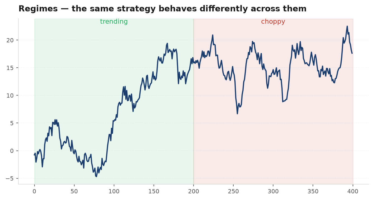
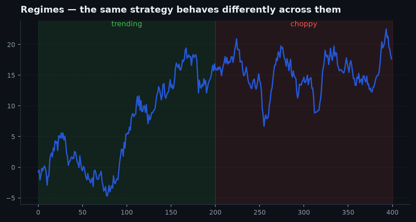
The observable symptom of a regime is a shift in the statistics of returns, not the returns themselves. Two regimes worth separating recur everywhere:

Calm vs volatile. The clearest and most robust split. Volatility clusters (you saw this with GARCH), so the market spends stretches in a low-variance state and stretches in a high-variance state, with sharp transitions between them. Risk sizing lives or dies on getting this right.
Trending vs choppy. A directional-persistence split: in a trend, moves autocorrelate and momentum pays; in a range, moves reverse and fading pays. Harder to detect cleanly than the vol split, because the difference is in the sign structure, not the magnitude.

The modelling assumption that makes this tractable: the regime is a hidden discrete state that you cannot observe directly, but which changes the distribution of the returns you can observe. Estimate the state from the observations and you have a regime detector.

A return series whose volatility and mean visibly shift between two regimes — A series that switches between a calm regime (tight, low-variance fluctuations) and a volatile regime (wide swings). The regime is not directly labelled in the data — the job of a regime model is to recover the hidden state that generated each bar.

Markov chains and transition matrices#

The mathematical backbone is a Markov chain: a system that hops between a finite set of states, where the probability of the next state depends only on the current state — not the whole history. That memoryless property is the Markov assumption:

P (S_{t + 1} = j ∣ S_{t} = i, S_{t - 1}, \dots) = P (S_{t + 1} = j ∣ S_{t} = i) = A_{ij}

All the dynamics live in the transition matrix $A$ , whose entry $A_{ij}$ is the probability of moving from state $i$ to state $j$ . Each row sums to 1. For a two-state calm/volatile model it is just:

A = (A_{00} A_{10} A_{01} A_{11}), A_{i 0} + A_{i 1} = 1

The diagonal entries are the persistence of each regime. A calm state with $A_{00} = 0.97$ stays calm 97% of bars, so its expected duration is $1/ (1 - A_{00}) \approx 33$ bars. High diagonal values are what make regimes sticky — long runs rather than bar-to-bar flip-flopping — which is exactly the realistic behaviour you want a detector to reproduce.

✦Scenario: reading durations off the transition matrix

A fit on daily equity returns hands back

A = (0.97 0.10 0.03 0.90)

. Read it as expected durations. The calm state (row 0) persists with

A_{00} = 0.97

, so once calm it stays calm for

1/ (1 - 0.97) \approx 33

trading days — about a month and a half of quiet. The volatile state (row 1) persists with

A_{11} = 0.90

, an expected

1/ (1 - 0.90) = 10

days — storms are shorter than calms, which matches how markets actually behave. And

A_{01} = 0.03

says that on any given calm day there is only a 3% chance of tipping into turmoil tomorrow. Those numbers are what stop a detector from flip-flopping regime every other bar — the stickiness is baked into the matrix.

The two-state Gaussian HMM#

A hidden Markov modelmakes the state unobserved and ties each state to a distribution over the observations. In the Gaussian two-state version, each bar's return is drawn from one of two normal distributions — one for each regime — and which one is chosen follows the Markov chain above:

S_{t} \in {0, 1} (hidden), x_{t} ∣ S_{t} = k \sim N (μ_{k}, σ_{k}^{2})

So the model has three sets of parameters: the two state means $μ_{0}, μ_{1}$ , the two state variances $σ_{0}^{2}, σ_{1}^{2}$ , and the transition matrix $A$ . Fit to returns, it typically discovers one low-variance state and one high-variance state — the calm/volatile split — without ever being told the labels.

Baum-Welch: fitting without labels#

You never observe the states, so you cannot fit by counting. The Baum-Welch algorithm (the expectation-maximisation instance for HMMs) solves the chicken-and-egg problem by iterating:

E-step (forward-backward). Given the current parameters, compute the posterior probability that each bar was in each state — the responsibilities $γ_{t} (k)$ .
M-step. Given those soft state assignments, re-estimate the means, variances, and transition matrix as probability-weighted averages.

Iterate to convergence and the parameters settle on a local maximum of the likelihood. edgekit's hmm_two_state implements this in pure numpy with scaled forward-backward for numerical stability, initialises the two means at the low and high quantiles of the data (so state 0 = low, state 1 = high for identifiability), and uses sticky initial transitions so it prefers long runs over rapid flipping:

import edgekit as ek

rets = ek.timeseries.log_returns(bars.close)

h = ek.timeseries.hmm_two_state(rets, iters=100, seed=0)
# h == {"states": ndarray of 0/1,   # the argmax-posterior regime path
#       "means":  [mu0, mu1],        # state means (state 0 low, state 1 high)
#       "vars":   [var0, var1],      # state variances
#       "trans":  2x2 row-stochastic transition matrix A,
#       "prob":   ndarray}           # posterior P(state 1) per bar, in [0,1]

print("regime means:", h["means"])
print("persistence (diagonal):", h["trans"][0][0], h["trans"][1][1])

The prob array — the posterior probability of being in the high state at each bar — is more useful than the hard states path, because it is a continuous confidence you can threshold or size against rather than a brittle 0/1 flip.

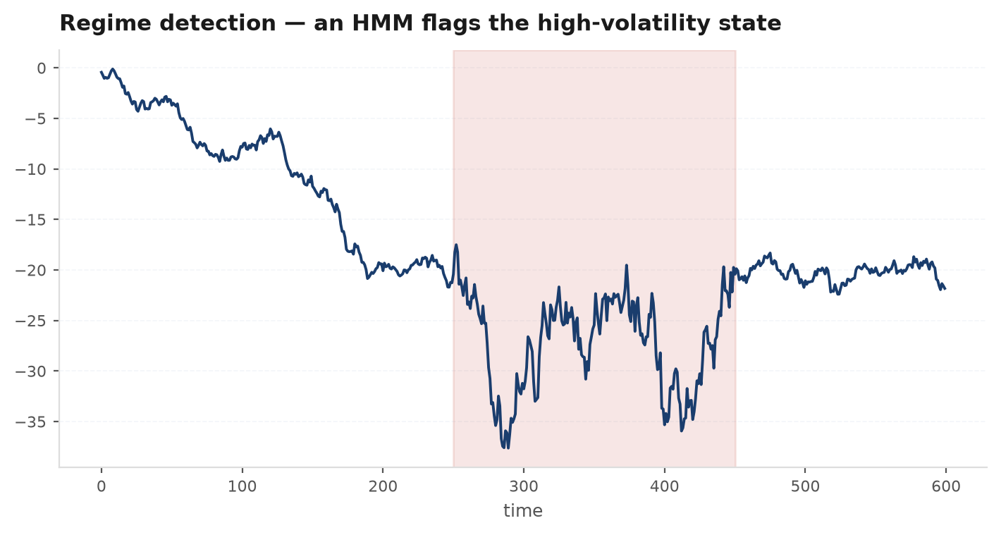
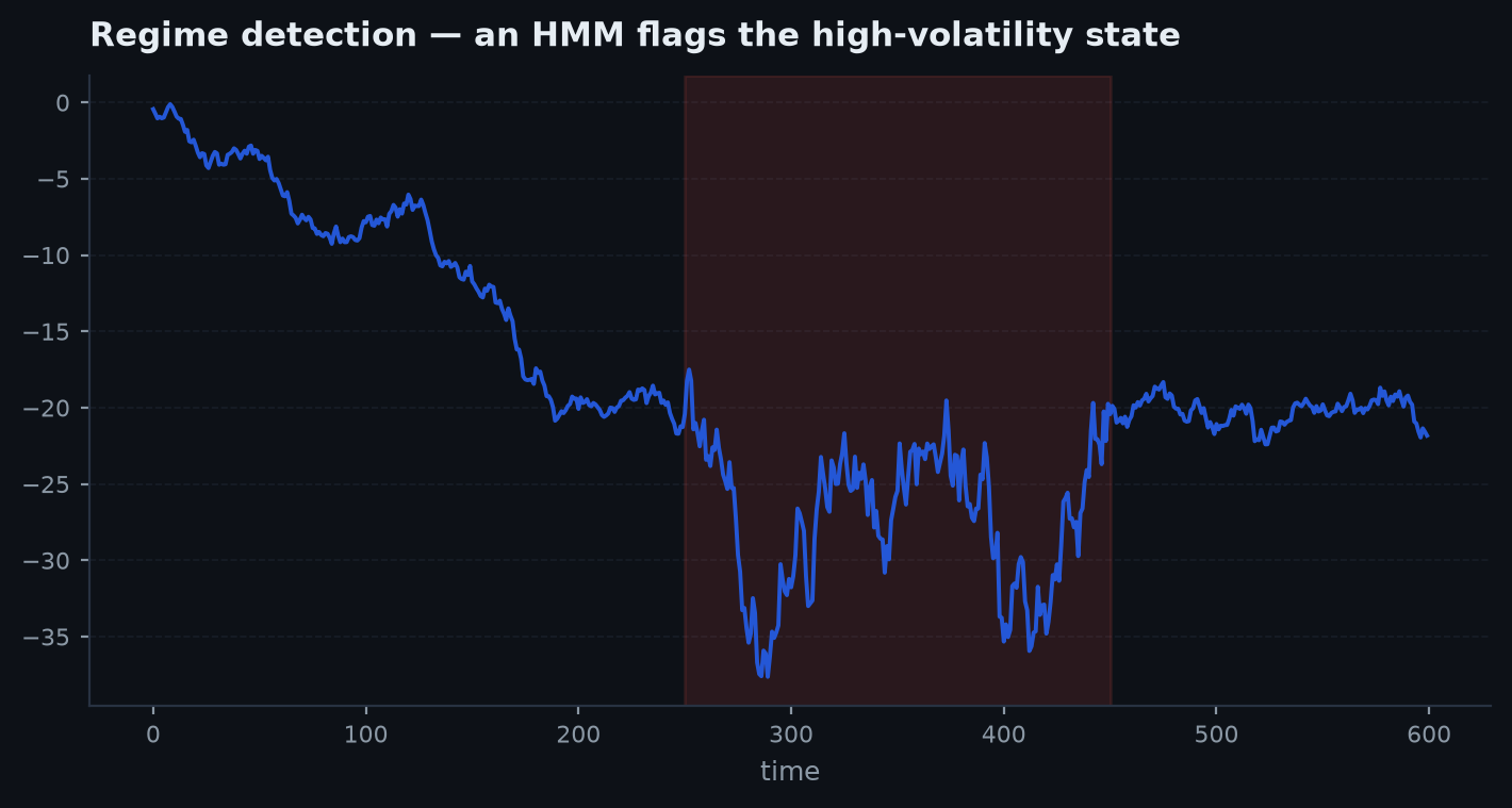
A price series shaded by the HMM-inferred regime with the posterior probability below — Top: the series with bars shaded by the HMM's inferred regime (calm vs volatile). Bottom: the posterior probability of the high-variance state — a continuous signal that ramps through transitions rather than snapping, which is what you actually gate risk on.

✦Scenario: the HMM flags a volatile month

Fit hmm_two_stateto daily S&P 500 returns and, without ever being told the labels, it discovers two states: state 0 with

μ_{0} \approx + 0.05%, σ_{0} \approx 0.7%

(calm, gently drifting up) and state 1 with

μ_{1} \approx - 0.10%, σ_{1} \approx 2.4%

(volatile, negative-drift — the crash signature). Through most of the sample h["prob"] — the posterior probability of the high-variance state — sits near 0.05. Then, in one month, it ramps over three or four days from 0.1 to above 0.9 and stays pinned there for ~15 bars before decaying back. That elevated stretch is the volatile month, flagged bar by bar from the returns alone. Note the ramp: the continuous prob starts warning you during the transition, which is exactly the early signal you want — far more useful than the hard 0/1 states flip that only commits after the fact.

Using the regime#

Once you have a regime label or probability, there are two clean ways to spend it, both risk overlays on an already-validated edge:

Gate the strategy. Turn a model on only in the regime where it has an edge — e.g. allow a mean-reversion pair to trade only when $P (volatile) < 0.5$ , and stand aside in the high-vol state where reversion breaks down.
Scale the risk.Keep trading in both regimes but shrink size when the volatile-state probability is high. Because the HMM's high state is the high-variance state, this is a discrete cousin of the continuous volatility targeting from the GARCH chapter.

# gate a signal by the inferred regime (posterior of the high-vol state)
h = ek.timeseries.hmm_two_state(rets, iters=100, seed=0)
p_high = h["prob"]                    # P(volatile) per bar

# inside a BaseStrategy: only take entries when the calm-regime probability is high
def regime_ok(t):
    return p_high[t] < 0.5            # stand aside in the volatile regime

# or scale exposure continuously: size_multiplier = 1 - p_high[t]

✦Scenario: gating the pair that blew up in the hook

Take the mean-reversion pair from the opening hook and gate it on this regime signal. In the calm state (

p_{high} < 0.5

) it trades normally and harvests the reversion it is good at. When p_high ramped above 0.5 heading into that ugly autumn week, regime_ok would have returned False and stood the pair down — sitting out precisely the trending stretch that ran it over. The continuous alternative,

size = 1 - p_{high}

, is gentler: it does not slam the book shut, it fades exposure toward zero as conviction that the regime has turned rises. Either way the regime label is spent as a risk overlay on an edge you already validated — never as the edge itself.

→The high state maps to what you fit it on

Fit the HMM to returns and the two states separate by variance (calm vs volatile). Fit it to a trend proxy — say a rolling return or an ADX-like series — and the states separate by direction/trend strength instead. The model finds structure in whatever series you hand it, so choose the input to match the regime you actually care about.

Change-point detection: the other framing#

An HMM answers “which of these recurring states am I in?” A complementary question is “when did the statistics break?” — change-point detection. Instead of a fixed set of states with return transitions, you scan for the moment the mean or variance of the series shifts, by comparing the likelihood of “one distribution throughout” against “a distribution that switches at time $τ$ .” The two views are close cousins: a change point is a transition in a model with non-recurring states. Change-point framing is the natural tool when regimes do not recur — a one-way structural break like a market microstructure change — whereas the HMM is right when calm and volatile keep alternating.

The two ways regime models lie to you#

Regime detection is uniquely seductive and uniquely dangerous, for two reasons that both amount to smuggling the future into the past.

✕Look-ahead in the labels

The Baum-Welch fit above uses the entire series to label every bar — the regime at bar

t

is informed by data from

t + 1, t + 2, \dots

. That is a perfect in-sample chart and a fantasy in live trading, where you only have the past. To use a regime label in a backtest honestly you must re-fit (or at least re-infer) using only data available at each bar — an expanding or rolling fit — and accept that the causal label is laggier and noisier than the smoothed one. A strategy that looks brilliant on full-sample regime labels and mediocre on causal ones was trading the future.

✕Overfitting the regimes

With enough states, means, and variances, an HMM can carve any history into tidy regimes that “explain” every drawdown after the fact — and generalise to nothing. Two disciplines keep you honest: prefer the fewest states that capture a real economic distinction (two is usually plenty), and validate the gated strategy out-of-sample, not the regime fit. If the regime does not survive on data the model never saw, it was a story, not a signal. Take it through the gauntlet like anything else.

Next: Risk management — regimes tell you when risk is elevated; this final chapter of the part turns that into concrete controls: Value-at-Risk and its critiques, Expected Shortfall as a coherent tail measure, drawdown and the ulcer index, risk budgeting, and sizing to a risk target.