Random matrix theory

Estimate a correlation matrix for 100 assets from a year of daily data and most of what you get is noise — structured, plausible-looking noise that an optimizer will happily leverage into a portfolio. Random matrix theory supplies the antidote: an exact description of what the eigenvalue spectrum of pure noise looks like, so anything inside that envelope can be discarded and anything outside it — the market mode, the sectors — can be kept. It is the multiple-testing correction of linear algebra: a null distribution for eigenvalues.

✦Intuition — why more assets makes estimation worse, not better

A correlation matrix for $N$ assets holds $N (N - 1) /2$ distinct numbers. For $N = 100$ that is 4,950 correlations — estimated from $T = 252$ days, i.e. about 25,000 data points. Five data points per parameter. Each individual correlation is merely fuzzy, but an optimizer does not read them individually: it hunts through all 4,950 at once for the combination that looks most diversifying — and with five points per parameter, the best-looking combination is almost always a sampling fluke. This is the same trap as testing 4,950 strategies and funding the best backtest. What you need is exactly what the gauntlet gave you for backtests: the distribution of what pure luck produces. For eigenvalues, that distribution has a name — Marchenko-Pastur — and a closed form.

The estimation problem: N/T is not small#

Classical statistics lives in the limit $T \to \infty$ with $N$ fixed, where the sample covariance converges to the truth. Portfolios live elsewhere: $N = 100$ assets, $T = 252$ days, so the ratio

q = \frac{N}{T} = \frac{100}{252} \approx 0.40

is order one, and stays order one no matter how you grow the universe (more history means older, staler regimes — you cannot just crank $T$ ). In this regime the sample covariance is not a noisy version of the truth; it is systematically distorted: sample eigenvalues spread out around the true ones — the largest biased up, the smallest biased down. The smallest-eigenvalue directions are precisely the ones a minimum-variance optimizer loads up on (“look, a riskless combination!”), which is why naive Markowitz out of sample is an error maximizer: it invests most where the estimate is worst, as Part VI’s optimization chapter warned.

The Marchenko-Pastur law#

Random matrix theory answers the null question exactly. Take $T$ observations of $N$ truly independent unit-variance series — pure noise, true correlation matrix $= I$ , all true eigenvalues equal to 1 — and form the sample correlation matrix. As $N, T \to \infty$ with $q = N / T$ fixed, its eigenvalue histogram converges to the Marchenko-Pastur density

ρ (λ) = \frac{1}{2 π q} \frac{( λ _{+} - λ ) ( λ - λ _{-} )}{λ}, λ_{\pm} = (1 \pm q)^{2} = (1 \pm N / T)^{2},

supported only on $[λ_{-}, λ_{+}]$ . Read what it says: even though every true eigenvalue is exactly 1, the sample eigenvalues smear across a whole interval — for $q = 0.4$ , from about 0.14 up to about 2.66. That smear is created by estimation alone. Any eigenvalue of a real correlation matrix that lands inside $[λ_{-}, λ_{+}]$ is indistinguishable from noise; only eigenvalues above $λ_{+}$ carry evidence of true correlation structure. The MP edge is the significance threshold for factors.

✦Derivation — the spread is exactly q, by trace bookkeeping

Two moments of the MP law follow from bookkeeping alone, no heavy machinery. First, the trace of a correlation matrix is $N$ (ones on the diagonal), and the trace is the sum of eigenvalues — so the average sample eigenvalue is exactly 1, noise or not:

λ = \frac{1}{N} tr (C) = 1.

Second, the average squared eigenvalue is $\frac{1}{N} tr (C^{2}) = \frac{1}{N} \sum_{i, j} C_{ij}^{2}$ — ones on the diagonal plus $N (N - 1)$ squared off-diagonal entries. For independent series, each sample correlation has variance $\approx 1/ T$ , so

λ^{2} \approx \frac{1}{N} (N + N (N - 1) \cdot \frac{1}{T}) \approx 1 + q, Var (λ) = λ^{2} - λ^{2} \approx q .

Why it matters: the eigenvalue spread of pure noise has variance $q = N / T$ — it comes entirely from the tiny $1/ T$ errors in each pairwise correlation, aggregated across $N^{2}$ of them. The distortion is not a flaw in your estimator; it is the unavoidable arithmetic of estimating quadratically many parameters from linearly much data. Only the ratio $N / T$ can shrink it, and in live portfolios $N / T$ is never small.

The law is easy to see for yourself — correlate pure noise and look at the spectrum:

mp_null.py

import numpy as np

rng = np.random.default_rng(11)
N, T = 100, 252
q = N / T

X = rng.standard_normal((T, N))          # T obs of N independent series: zero true structure
evals = np.linalg.eigvalsh(np.corrcoef(X, rowvar=False))

lam_plus = (1 + np.sqrt(q)) ** 2          # ~ 2.66: the MP noise ceiling
evals.min(), evals.max()                  # ~ (0.14, 2.66) -- the full MP smear from nothing
(evals > lam_plus).sum()                  # ~ 0: no true factors, none detected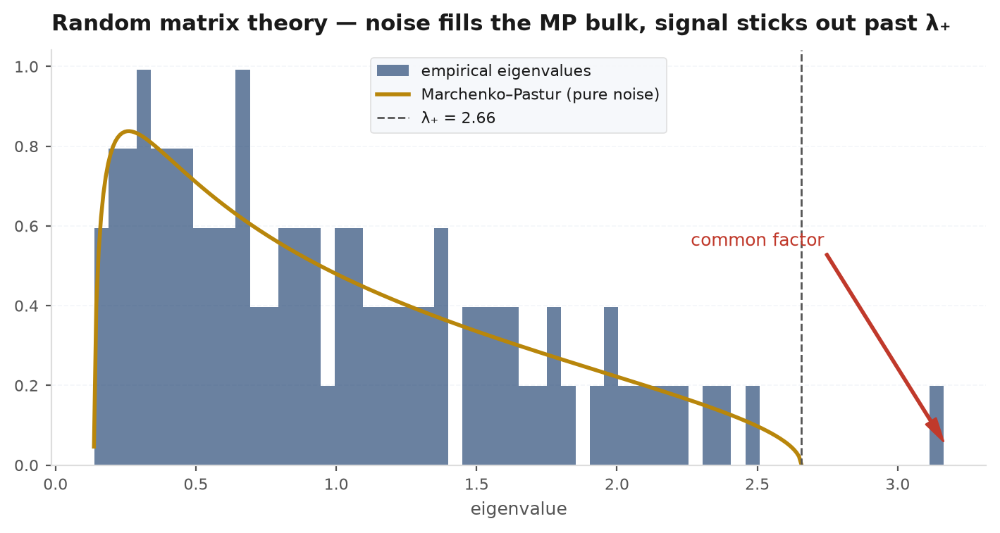

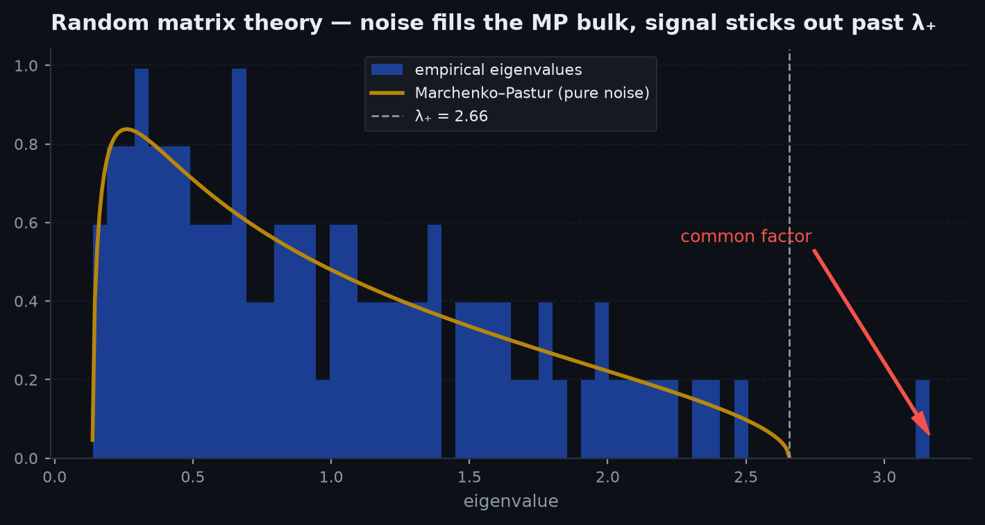
Histogram of sample correlation eigenvalues with the Marchenko-Pastur density overlaid on the noise bulk, and a few large outlier eigenvalues including the market mode standing far above the upper edge — Eigenvalue spectrum of an equity correlation matrix vs the Marchenko-Pastur null (curve). The bulk of eigenvalues hugs the MP density — statistically pure noise. A handful escape above the edge lambda_+: sector factors just outside, and far to the right the market mode, an eigenvalue an order of magnitude above the bulk.

✦Scenario — N = 100, T = 252: where is the noise line?

The house case: $N = 100$ assets, one year of daily data, $T = 252$ . Then $q = 100/252 \approx 0.63$ and the noise bulk spans

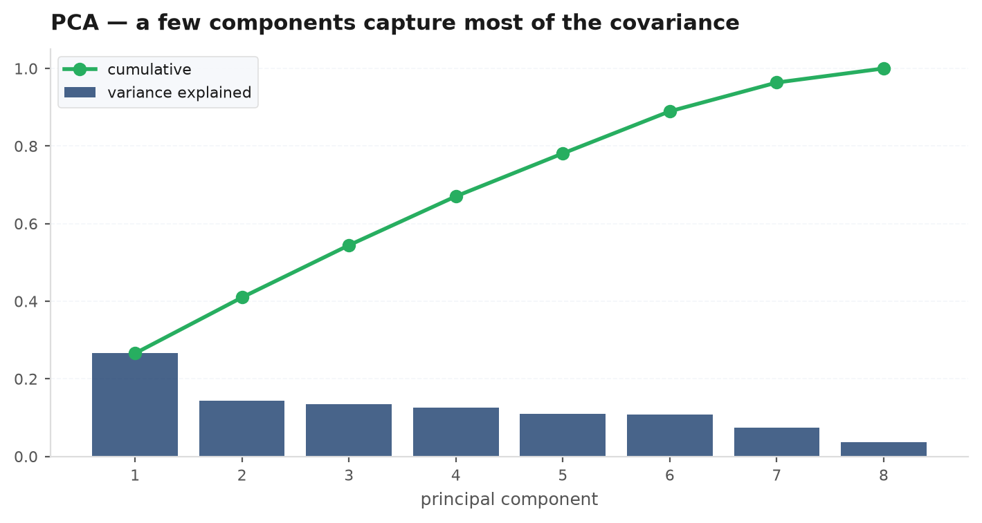
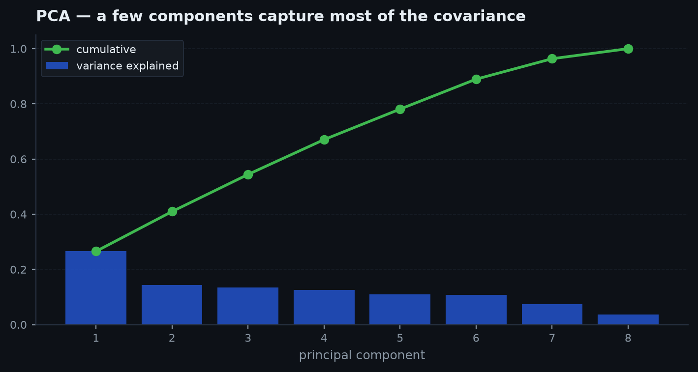
λ_{-} = (1 - 0.63)^{2} \approx 0.14, λ_{+} = (1 + 0.63)^{2} \approx 2.66.

An eigenvalue must exceed roughly $2.7$ — carry nearly three timesan average asset’s share of variance — before it means anything at all. In a typical equity universe that leaves perhaps 5–10 survivors out of 100: the market mode (eigenvalue $\approx N ρ ˉ \approx 30$ for average correlation $ρ ˉ \approx 0.3$ — a tenth of a 100-asset universe’s variance riding one direction) and a handful of sector factors in the 3–10 range. The other ~90 eigenvalues — 90% of the matrix’s dimensions, the ones encoding all those tempting fine-grained hedges — are statistically indistinguishable from what you would get correlating 100 streams of white noise. Every optimizer decision built on them is curve-fitting.

Scree plot of variance explained by principal components of an asset return correlation matrix, with one dominant component, a few moderate ones, and a long flat tail — The same story as a PCA scree plot: one dominant component (the market), a few meaningful ones (sectors), then a long flat tail. RMT turns this picture quantitative — the MP edge says exactly where the meaningful components end and the flat tail of noise begins.

Cleaning the matrix: clipping vs shrinkage#

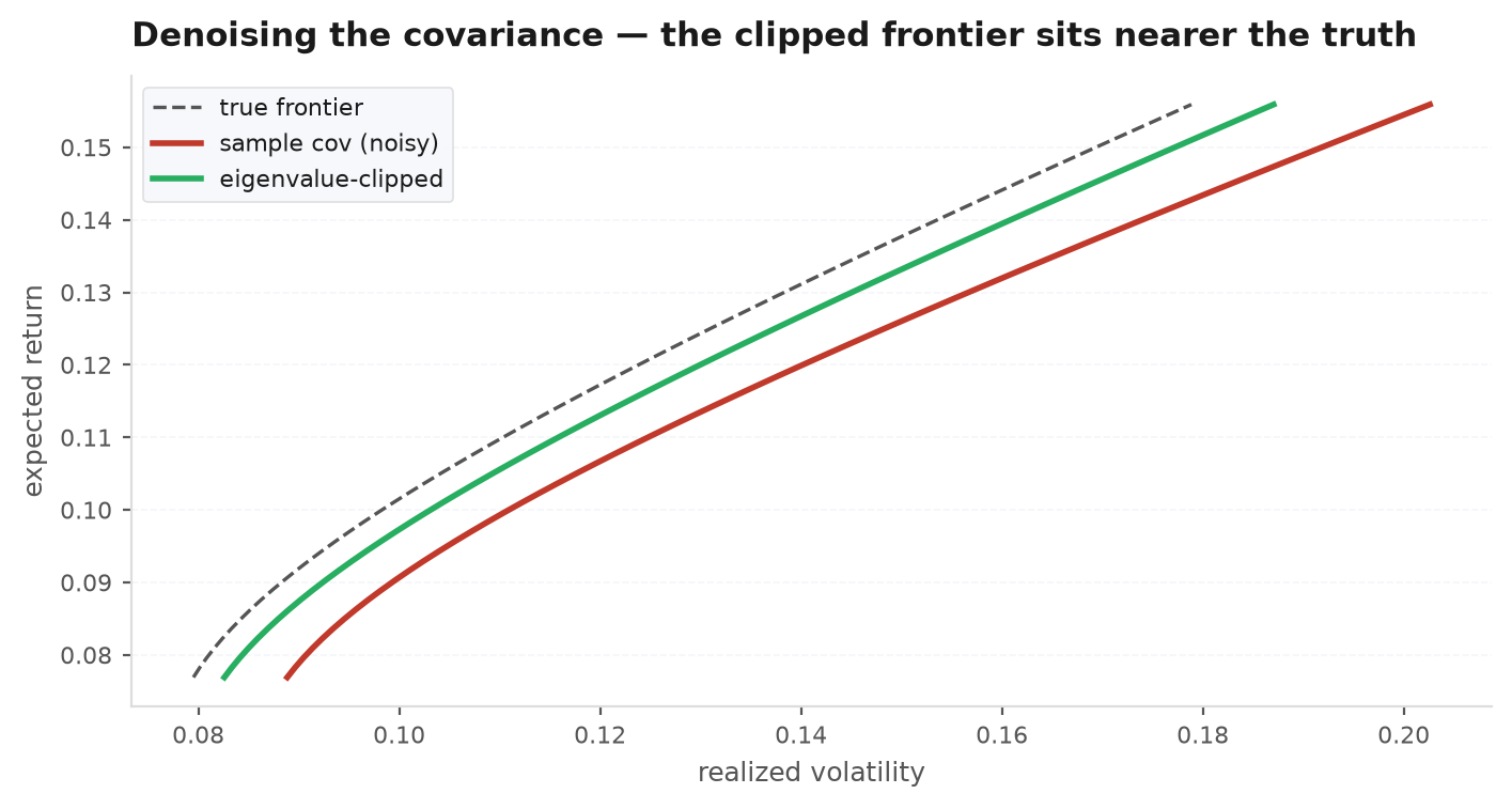
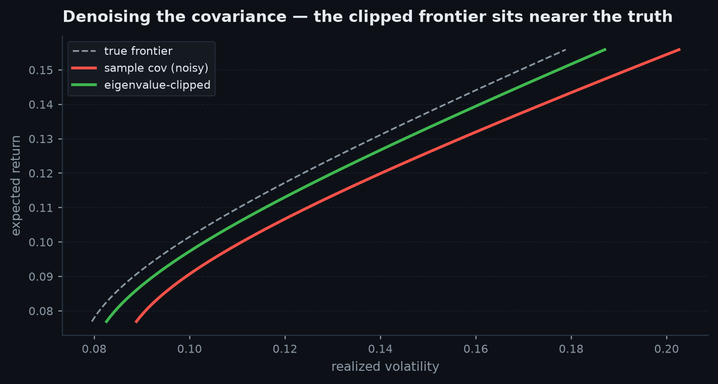
Two families of fixes, both keeping the eigenvectors and repairing the eigenvalues. Eigenvalue clipping (MP denoising) is surgical: keep every eigenvalue above $λ_{+}$ as measured, and replace all eigenvalues below it by their common average (preserving the trace, i.e. total variance), flattening the noise bulk back toward the identity it statistically is. Reassemble $C^{'} = V Λ^{'} V^{⊤}$ , rescale the diagonal to ones, done:

denoise.py

import edgekit as ek

corr = returns.corr().to_numpy()            # N x N sample correlation, T rows in returns

# Marchenko-Pastur clipping: eigenvalues below lambda_+ are noise -> averaged.
corr_mp = ek.optimize.mp_denoise(corr, n_obs=len(returns))

# Ledoit-Wolf: shrink the sample covariance toward a structured target,
# with the shrinkage intensity chosen optimally from the data itself.
cov_lw = ek.optimize.ledoit_wolf(returns)

# Same optimizer, three inputs -- compare the weights they produce:
w_raw = ek.optimize.min_variance(ek.optimize.sample_cov(returns))
w_lw  = ek.optimize.min_variance(cov_lw)
# (and min_variance on the vol-rescaled corr_mp) -- raw weights are extreme
# and flip sign across resamples; cleaned weights are stable and spread out.

Ledoit-Wolf shrinkage is statistical rather than spectral: replace the sample covariance $Σ^$ with a convex blend $Σ_{LW} = α F + (1 - α) Σ^$ toward a simple target $F$ (identity, or constant correlation), with the intensity $α$ chosen by an explicit formula that minimises expected estimation error — more data or less noise, less shrinkage. It is the Bayesian move (pull noisy estimates toward a prior) applied to a whole matrix. In the eigenvalue picture, shrinkage squeezes all eigenvalues toward the centre proportionally, while clipping flattens the bulk exactly and leaves the outliers untouched. In practice: clipping is more aggressive on the noise floor and keeps sector structure crisp; Ledoit-Wolf is smoother, never produces a singular matrix, and needs no threshold. Both beat the raw matrix out of sample, essentially always; which of the two wins is second-order compared to using either.

Realized out-of-sample efficient frontiers built from the raw sample covariance versus the Marchenko-Pastur denoised covariance, with the denoised frontier dominating and the raw frontier far below its promised in-sample position — Out-of-sample frontiers: portfolios optimized on the raw sample covariance vs the MP-denoised one. The raw optimizer's frontier promised more in-sample (it fit the noise) and delivers less out-of-sample; the denoised frontier gives up fictional in-sample efficiency and dominates where it counts.

Eigenportfolios#

The surviving eigenvectors are portfolios. Eigenvector $v_{k}$ defines the eigenportfolio with weights proportional to $v_{k}$ (normalised), and the eigenvalue $λ_{k}$ is that portfolio’s variance in correlation units — eigenportfolios are uncorrelated with each other by construction. The first is the market: all weights the same sign, roughly equal — its return is essentially the index, and $λ_{1} / N$ is the fraction of total variance the market factor commands. The next few are long-short sectorspreads (long energy, short tech). Everything below the MP edge is an unstable direction that will reshuffle completely in the next sample — treating those as tradable “factors” is fitting noise. This gives statistical arbitrage its standard decomposition: project returns on the significant eigenportfolios, call that the systematic part, and trade the residual — mean-reversion machinery of pairs trading generalised to a whole universe, with RMT deciding how many factors to strip.

The working recipe#

Compute the edge first. $λ_{+} = (1 + N / T)^{2}$ before you look at the spectrum — decide the threshold before seeing the data, exactly as with any hypothesis test.
Count survivors, not components. Keep eigenvalues above $λ_{+}$ ; expect a market mode plus a handful of sectors, and be suspicious of anything barely over the line.
Clean before you optimize. mp_denoise or ledoit_wolf on the way into any optimizer — never the raw sample matrix for $N / T ≳ 0.1$ .
Judge out of sample. The only test that counts is realized variance of the resulting weights on unseen data — the cleaned matrix should win, and does.

Assumptions vs reality#

RMT assumes	Reality	Consequence
i.i.d. returns over time	Volatility clustering, autocorrelation	Effective T is smaller; the true noise band is wider than MP
Gaussian-ish entries	Fat tails	Heavy tails fatten the bulk edge; a few big days can fake an outlier
N, T large (asymptotic law)	Finite samples	Edge is fuzzy (Tracy-Widom): eigenvalues just above lambda_+ are marginal
Stationary correlations	Correlations spike toward 1 in crises	The market mode grows exactly when diversification is needed most

!An eigenvalue just above the edge is a maybe, not a factor

The MP edge is an asymptotic statement; in finite samples the largest noise eigenvalue fluctuates around

λ_{+}

(Tracy-Widom fluctuations), and fat tails plus volatility clustering push it higher still. Treat eigenvalues at

1.1 \times

the edge as suspects, not factors — and confirm any borderline factor the same way you confirm any edge: does it persist out of sample? The eigenvector of a marginal eigenvalue typically rotates completely between adjacent years, which is the spectral version of a backtest that fails walk-forward.

Next: cleaned covariance in hand, the question becomes what to do with it — constraints, resampling, and turnover-aware weights in Portfolio construction.