Portfolio construction

One validated strategy is a business with a single point of failure. Two strategies whose returns don't move together are a portfolio whose combined risk is less than the sum of its parts — the only free lunch in finance. This chapter is the math of that lunch: portfolio variance, correlation, and the weighting schemes (equal-weight, inverse-vol, risk parity, HRP) that turn a set of independent books into one steadier equity curve.

Start from scratch with two market stalls on the same street. One sells umbrellas, one sells sunglasses. Each on its own has wild months — the umbrella seller starves in a drought, the sunglasses seller in a monsoon. But own bothand your street income barely moves with the weather: when one is quiet the other is busy. You did not raise your average takings; you smoothed them — and a smoother income at the same average is worth strictly more, because you can size up on it, borrow against it, and sleep through it. Two trading strategies whose good and bad months don't line up are umbrellas and sunglasses. This chapter is the arithmetic of exactly how much smoother the street gets, and it all turns on one number: the correlation between the two.

Combining strategies into one book#

The unit of combination in edgekit is the daily-R series— each strategy's per-day sum of trade R-multiples, indexed by date. A day the strategy didn't trade contributes $0$ R, not missing data. ek.portfolio.combine merges the per-strategy series onto one date grid and applies a weighting method:

combine(books: dict[str, pd.Series], method="risk_parity",
        weights=None) -> pd.Series
# method in "equal" | "fixed" | "risk_parity"

combine.py

from edgekit import portfolio

# r_trend, r_breakout: each a daily-R series from a validated strategy
book = portfolio.combine({"trend": r_trend, "breakout": r_breakout}, method="risk_parity")

The diversification math#

Why two books beat one comes straight out of the variance of a weighted sum. For weights $w_{i}$ , per-book volatilities $σ_{i}$ , and pairwise correlations $ρ_{ij}$ , the portfolio variance is:

σ_{p}^{2} = i \sum j \sum w_{i} w_{j} σ_{i} σ_{j} ρ_{ij}

The two-book case makes the mechanism obvious:

σ_{p}^{2} = w_{1}^{2} σ_{1}^{2} + w_{2}^{2} σ_{2}^{2} + 2 w_{1} w_{2} σ_{1} σ_{2} ρ_{12}

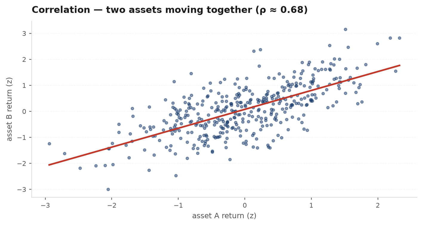
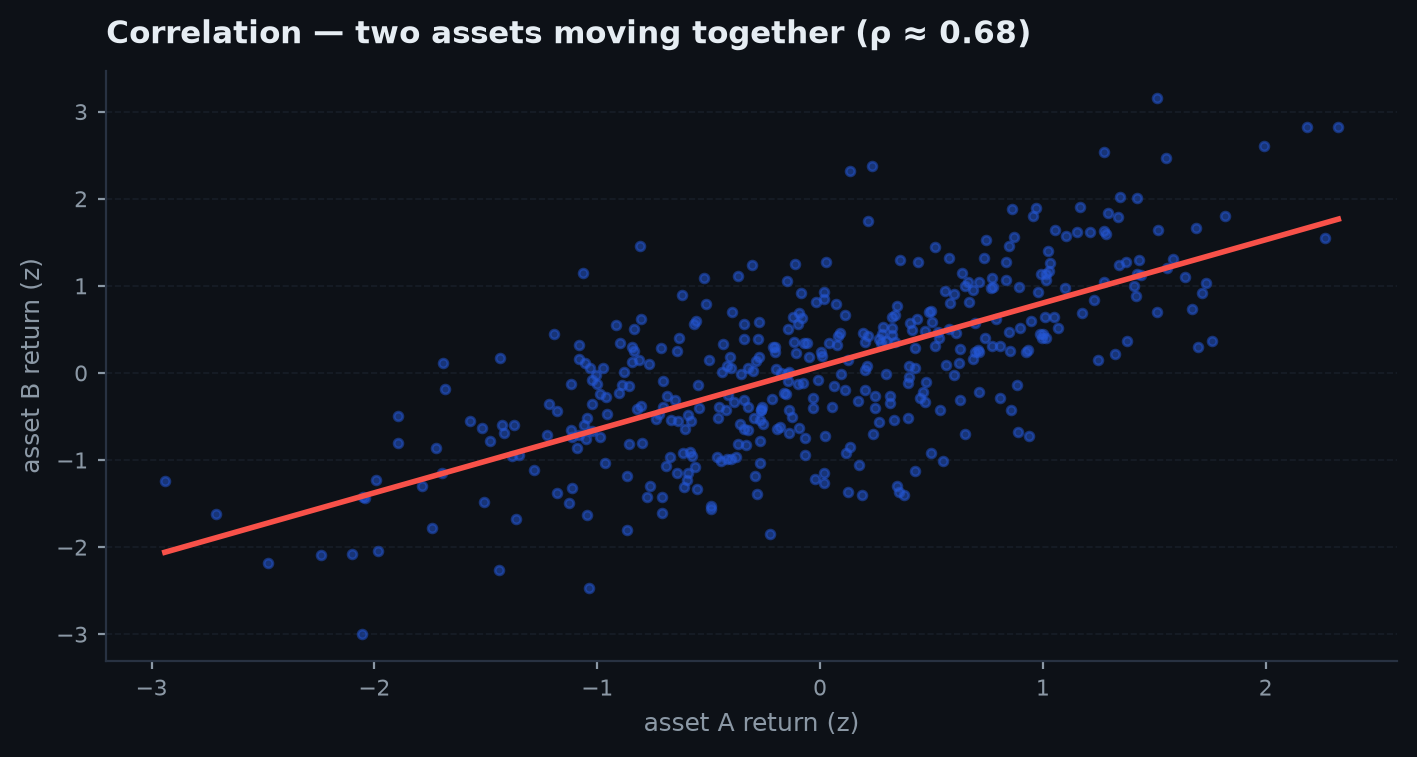
The cross term carries $ρ_{12}$ . If the books are uncorrelated ( $ρ_{12} = 0$ ) it vanishes, and combined volatility is $w_{1}^{2} σ_{1}^{2} + w_{2}^{2} σ_{2}^{2}$ — strictly less than the weighted sum of the two volatilities. If they are negatively correlated, the cross term is negative and risk falls further. The return of the combined book is just the weighted average of the two means — so lower risk at the same return means a higher Sharpe. That is the entire case for diversification.

Scenario: a trend book and a breakout book. You have two validated daily-R books. A SmaCross crypto trend book swings at $σ_{1} = 1.4 R$ per day; an ORB-style US100 breakout book is quieter at $σ_{2} = 0.9 R$ per day. One holds crypto for days at a time, the other is flat by every US close, so their daily-R correlation lands at $ρ_{12} = + 0.08$ — essentially unrelated. Blend them 50/50 and the two-book variance formula becomes:

σ_{p}^{2} = 0. 5^{2} (1.4)^{2} + 0. 5^{2} (0.9)^{2} + 2 (0.5) (0.5) (1.4) (0.9) (0.08) \approx 0.49 + 0.20 + 0.05 = 0.74

so $σ_{p} \approx 0.86 R$ per day — lower than either book on its own, while the combined return is simply the average of the two means. That is the free lunch as a concrete number. Now suppose the two books had instead been the same trend signal on two instruments, correlated at $ρ = 0.9$ : the cross term swells from 0.05 to $2 (0.5) (0.5) (1.4) (0.9) (0.9) \approx 0.57$ , portfolio vol climbs back to $\approx 1.12 R$ , and the smoothing all but vanishes. Same books, same returns — the whole difference is the correlation.

Scatter of two books' returns with a fitted line and the correlation coefficient — The number the whole chapter turns on. Each point is one period's paired returns for two books; ρ measures how tightly they track the fitted line. A near-zero cloud (left) is the diversifying pair whose cross term vanishes; a tight upward line (ρ near 1) is two books moving as one, and no smoothing to be had.

✦Correlation, not count, is what diversifies

Ten strategies that are really the same trend signal on ten instruments have

ρ \approx 1

and diversify almost nothing — the cross terms nearly reproduce the weighted sum. Two genuinely different edges (a trend book and a mean-reversion book) at

ρ \approx 0

do far more for risk-adjusted return than ten correlated ones.

Measuring correlation honestly#

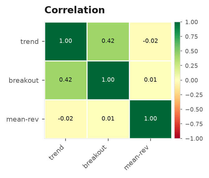
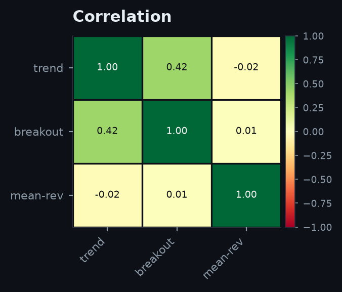
ek.portfolio.correlation returns the pairwise daily-R correlation matrix. It counts only days where at least one book was active — shared idle days (both flat at $0$ ) would pull the estimate spuriously toward zero and make two books look more diversifying than they are.

correlation.py

corr = portfolio.correlation({"trend": r_trend, "breakout": r_breakout})
print(corr.loc["trend", "breakout"])   # near 0 = genuine diversification

At the desk. Run correlation on the two books above and it prints $0.08$ — but only because it ignored the roughly 40% of calendar days when both books sat flat. Fold those shared zeros back in and a naive Pearson correlation sags toward $0.03$ , making the pair look more diversifying than it truly is. That is not a cosmetic difference: you size real risk against this number, and a spuriously low correlation quietly tells you to load up on a pair that will move together more than you budgeted for.

A correlation heatmap of several strategy books' daily-R series — Pairwise daily-R correlations. Cool off-diagonal cells are the pairs worth combining; a matrix that's warm everywhere is one strategy wearing many hats.

Weighting schemes#

Equal weight#

Give each book the same weight, $w_{i} = 1/ n$ . Simple and hard to overfit, but it lets a high-volatility book dominate the combined risk: a book with twice the vol contributes four times the variance. Equal capital is not equal risk.

Inverse-volatility (naive risk parity)#

Weight each book by the reciprocal of its volatility so every book contributes the same risk:

w_{i} = \frac{1/ σ _{i}}{\sum _{j} 1/ σ _{j}}

The quiet book gets the larger weight, the loud one is muted. ek.sizing.risk_parity builds these weights from a trailing volatility window — and every stat it uses is lagged one day (.shift(1)), so the weight on day $t$ only sees returns through $t - 1$ and never reads its own bar.

risk_parity.py

from edgekit import sizing

# M: DataFrame whose columns are per-book daily-R series
w = sizing.risk_parity(M, win=90)      # inverse-vol weights, each row sums to n_assets
book = (M * w).sum(axis=1)             # the equal-risk combined R-stream

This is exactly what combine(..., method="risk_parity")does under the hood. True risk parity — equalising each book's marginal contribution to portfolio risk, which accounts for correlations too — is the more complete version; inverse-vol is the robust, correlation-blind approximation that rarely does worse out-of-sample.

Scenario. Keep $σ_{1} = 1.4 R$ (trend) and $σ_{2} = 0.9 R$ (breakout). Inverse-vol weights are $w_{1} = (1/1.4) / (1/1.4 + 1/0.9) \approx 0.39$ and $w_{2} \approx 0.61$ : the quieter breakout book gets the larger share, precisely so each contributes the same risk to the blend. Equal capital (50/50) would instead let the louder trend book dominate the combined drawdown — the thing that actually breaches a limit — even while it holds only half the money.

Hierarchical Risk Parity (HRP)#

Classic mean-variance optimisation inverts the covariance matrix, which is wildly unstable on correlated books — tiny estimation errors produce enormous, concentrated weights. HRP (Lopez de Prado) sidesteps the inversion entirely: it clusters the books by correlation into a tree, then allocates risk top-down through the tree by inverse cluster-variance. The result is stable, diversified weights with no matrix inversion. ek.sizing.hrp is pure numpy and, like everything in the sizing layer, is strictly causal — day- $t$ weights are built only from the window before $t$ .

hrp.py

from edgekit import sizing
w = sizing.hrp(M, lookback=252, step=21)   # correlation-clustered risk weights
book = (M * w).sum(axis=1)

Choosing the split: allocation_sweep#

Between two books there is a whole family of blends. ek.portfolio.allocation_sweep sweeps the risk-share of book A, sizes each blend to the same drawdown budget, and reports both the return-maximising split and the robust risk-parity (50/50) default. Crucially, it can fix weights on an in-sample window and report what they did out-of-sample — because the best in-sample share is always optimistic.

allocation_sweep(book_a, book_b, dd_budget, daily_cap, account,
                 grid=None, cut=None) -> dict

allocation_sweep.py

res = portfolio.allocation_sweep(r_trend, r_breakout, dd_budget=0.10,
                                 daily_cap=0.05, account=100_000, cut="2023-01-01")
print(res["best_share"])          # return-maximising share of A (in-sample, optimistic)
print(res["risk_parity"])         # robust 50/50 default
print(res["oos"]["oos_annual"])   # what the IS-fixed weights did on unseen data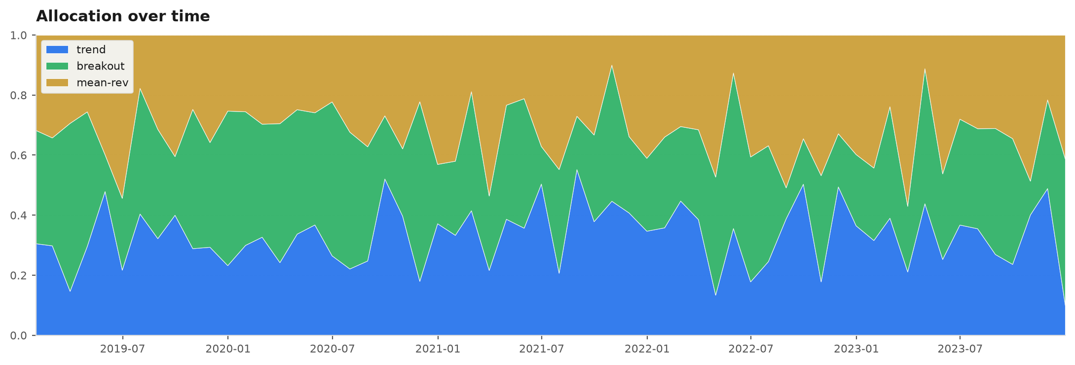

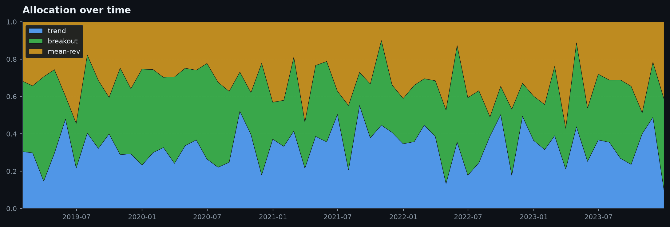
A stacked-area chart of each book's risk allocation across the sweep grid — Risk allocation across the blend grid. Read the OOS panel, not the in-sample peak — the return-maximising share is chosen on the same data it's measured on.

!Trust the OOS panel, not the best row

best_share is selected in-sample and therefore flatters itself. Pass a cut date and read the oos panel: it fixes 50/50 weights and sizing on the in-sample window and reports what they did on unseen data. If oos_annual collapses versus is_annual, the blend doesn't generalise — fall back to the correlation-blind risk-parity default, which has nothing to overfit.

Why correlation drifts — and why it matters#

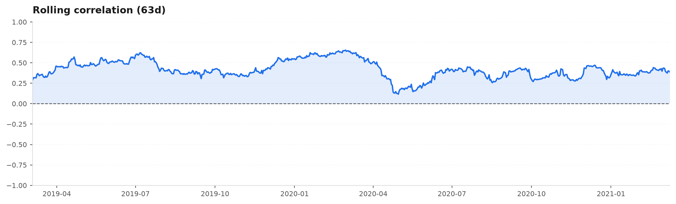
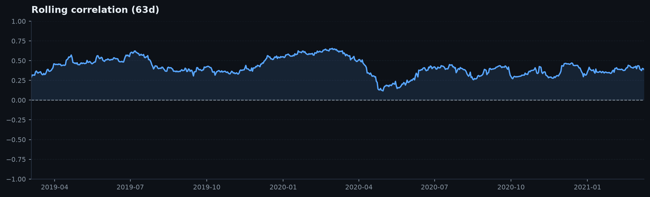
The diversification benefit is only as stable as the correlation that produces it. In a crisis, correlations across risk assets tend to spike toward $+ 1$ exactly when you most need them low — the cross term in the variance formula swells and the “free lunch” shrinks. Watch the rolling correlation, not just the full-sample number, so a pair that is diversifying on average but coupled in stress doesn't surprise you live.

Scenario: the correlation that moved.Through 2021–2023 the trend and breakout books above sit at a rolling $ρ \approx 0.05$ and the blend feels bomb-proof. Then a macro shock hits: crypto and the equity index sell off together, both books flip short into the same falling tape, and for six weeks their rolling correlation spikes to $0.6$ . The cross term you sized against at 0.05 is now more than ten times larger, the portfolio vol you budgeted for is blown through, and the drawdown lands deeper than the full-sample math ever suggested. This is why you size for the rolling peak, not the comfortable average — the diversification is only ever as reliable as its worst window.

Rolling pairwise correlation between two strategy books over time — Rolling correlation between two books. A full-sample rho near zero can hide windows where the pair moves together — size for the peaks, not the average.

Next: a combined book still has to survive a hard drawdown budget — Prop-firm and capital covers sizing to a drawdown limit and Monte-Carlo pass rates for funded-account evaluations.