Deep learning: a skeptic’s guide

Deep learning conquered vision, speech, and language — domains where it went from useless to superhuman inside a decade. It has not done that to daily-bar trading, and the reasons are structural, not a matter of waiting for a bigger model. This chapter is the case for skepticism: why the problem that made transformers great is almost the opposite of the problem a daily-frequency trader faces, where the failures actually hide, where deep models genuinely do earn their keep — and the honest protocol to follow if you insist on trying.

✦Intuition — why the vision playbook doesn’t transfer

A photo of a cat contains an enormous amount of signal about cat-ness: label noise is a rounding error, cats do not stop being cats because other people classified them, and a billion i.i.d. images are a billion real observations. Daily returns invert every one of those gifts. The signal is a whisper under a roar of noise; the patterns you learn are actively destroyed by the people who learn them; and a century of market history is, statistically, a handful of regimes in a trench coat. Deep nets are voracious signal extractors — hand one a dataset that is 99% noise and it will extract the noise, beautifully, with total conviction.

Signal-to-noise: the 1% problem#

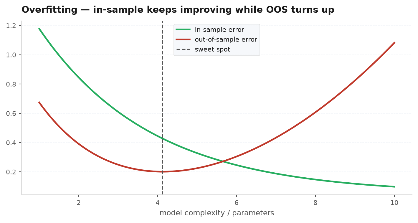
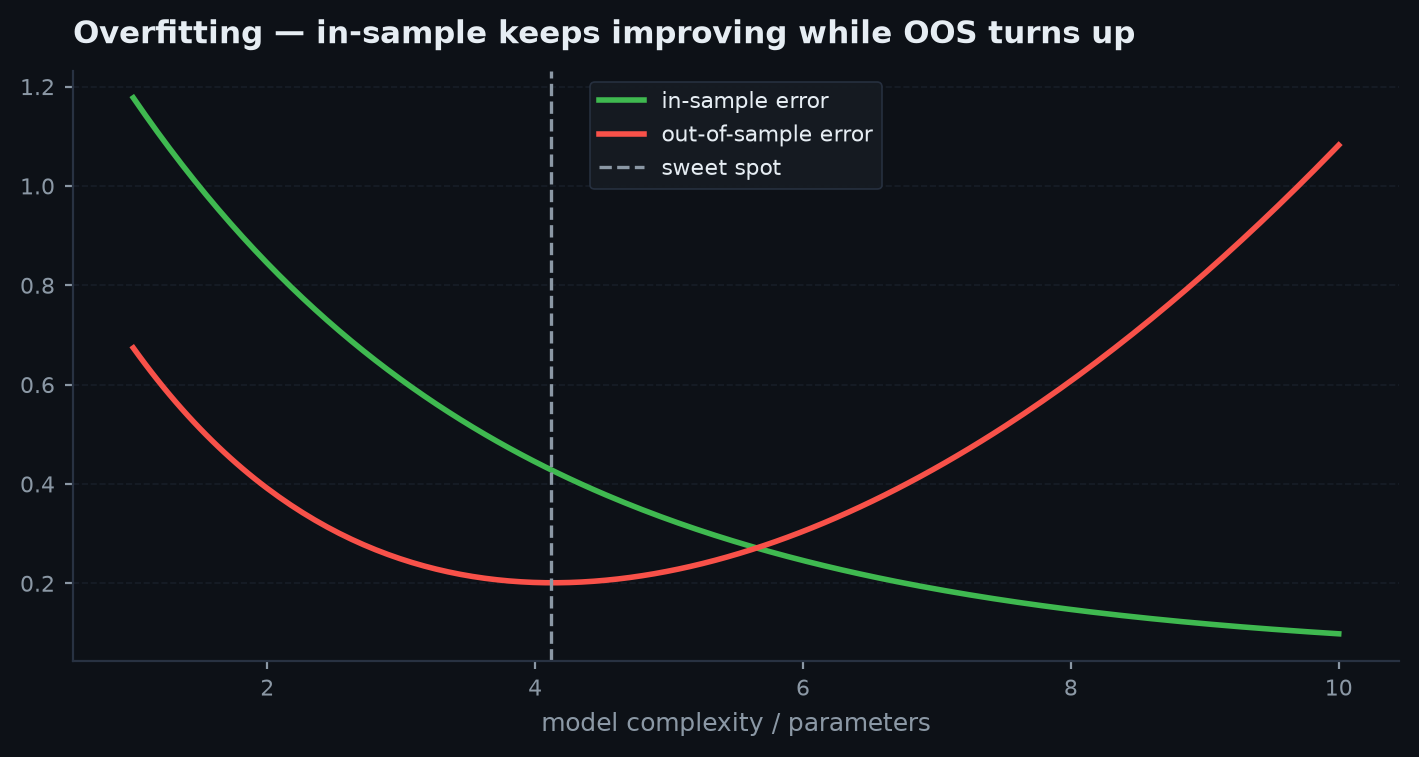
The best documented daily-horizon return predictors — the classic anomalies at their peak — deliver out-of-sample $R^{2}$ on the order of 1%, often less. That is the signal ceiling the market leaves un-arbitraged. Deep learning’s advantage is fitting complex functions, and the value of that advantage scales with how much structure exists to fit: at $R^{2} \approx 0.9$ (vision), a better function approximator is transformative; at $R^{2} \approx 0.01$ , the gap between a linear model and the true conditional mean is microscopic next to the noise, while the model’s extra capacity is a liability — millions of parameters with almost nothing real to explain will explain the unreal instead. This is overfitting at industrial scale.

Training error falling while validation error rises past the optimal complexity point — The familiar picture, from the overfitting chapter. Capacity beyond the signal's complexity fits noise. Deep nets start far to the right of a daily-bar problem's optimum — regularisation drags them left, but the prior is wrong from the start.

Non-stationarity: the distribution you trained on is gone#

Supervised learning’s core assumption is that training and deployment data share a distribution. Cats oblige; markets do not. Regimes shift (rates, microstructure, participants), and — worse — the map from pattern to profit is adversarial: any learnable structure attracts capital that erodes it, the edge-decaymechanism. A deep net’s millions of parameters encode a detailed portrait of the training era’s joint distribution; the more faithfully it memorises that world, the more specifically wrong it becomes when the world moves. Simple models degrade gracefully under drift; heavily parameterised ones can fail unrecognisably.

Effective sample size: decades are not big data#

Twenty-five years of daily bars is ~6,300 rows — and far fewer effectiveobservations. Overlapping feature windows make adjacent rows near-duplicates; volatility clustering correlates their errors; and at the level that matters for generalisation — distinct market regimes — the count is maybe a dozen. Training a 10M-parameter network on a dozen effective regime-observations is not machine learning, it is interpolation with extra steps. The domains where DL wins have sample counts (billions of tokens, millions of images) that exceed parameters or at least match the problem’s complexity. Finance at daily frequency simply does not — which is the first hint of where DL can work: frequencies where data is genuinely abundant.

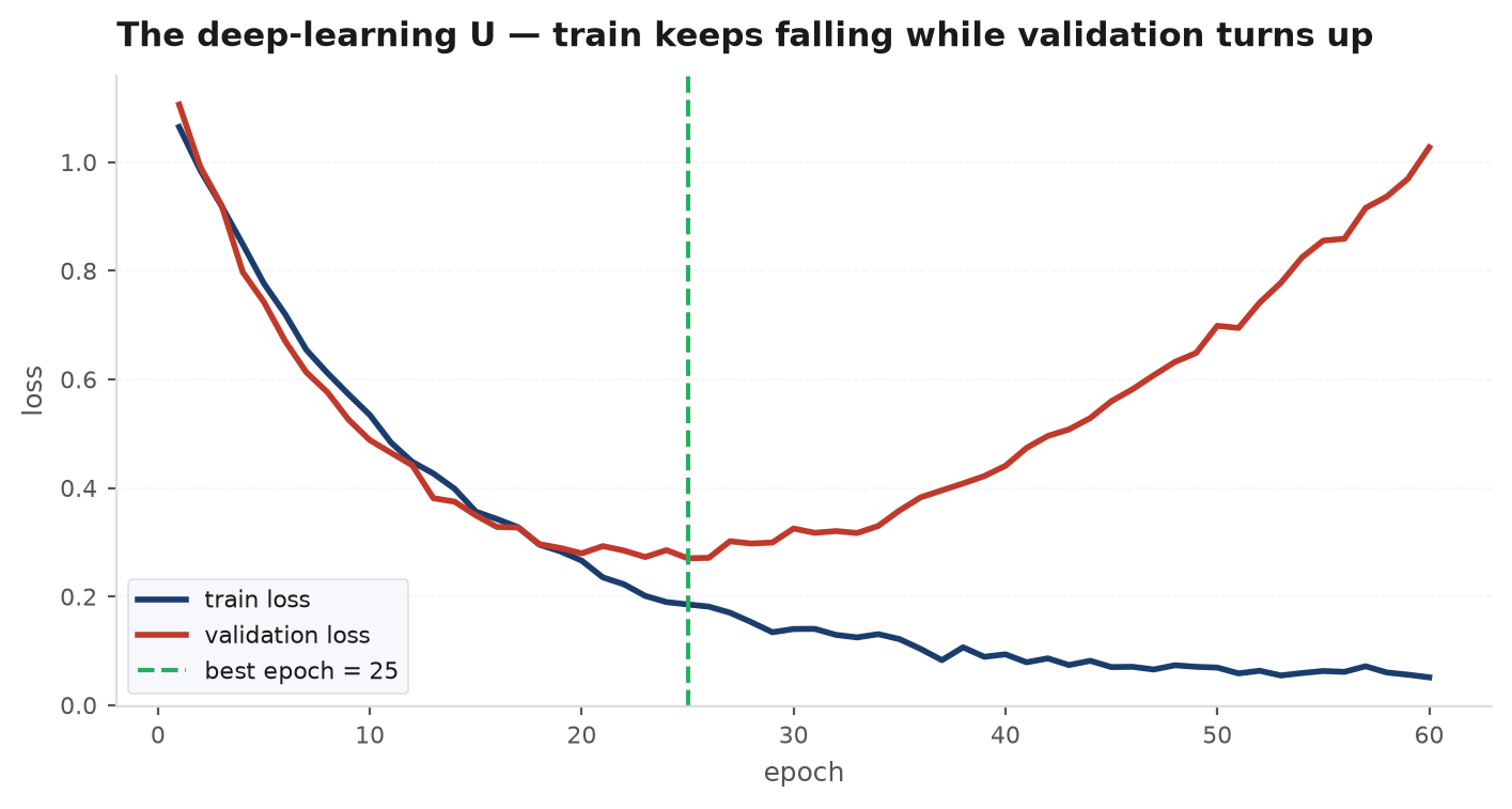
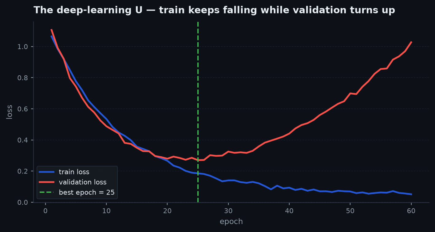
✦Scenario — actually count your effective n

Take a concrete setup: 25 years of daily bars on one index, features built from 60-day windows, labels with a 10-day horizon. The row count says $n = 6, 300$ . Now count what is actually independent. Adjacent rows share 59 of 60 feature days and 9 of 10 label days, so non-overlapping observations number roughly $6, 300/60 \approx 105$ . Those 105 windows are not i.i.d. either — they cluster into perhaps 8-12 volatility/rate regimes, and generalisation to the next regime is the thing you actually need. Compare the classic vision baseline: ~1.2m independent images for ~25m parameters, a ratio of about 1:20. A 100k-parameter net on ~100 effective observations is a ratio of 1:1,000 — fifty thousand timesworse — before the labels’ 1% signal content is even considered. This arithmetic, not any failure of optimisation, is why the training curve in the figure below can fall smoothly while out-of-sample performance stays pinned at zero.

Leakage by architecture#

Beyond the classic pitfalls, deep pipelines add leak paths of their own, each producing a validation curve that flatters:

Normalisation leaks. Scaling with statistics computed over the full dataset (or a BatchNorm layer mixing test-batch statistics) hands the model information from the future. Fit scalers on the training window only, per split.
Sequence-window leaks. Sliding windows whose input overlaps the label horizon of a neighbouring test sample leak outcomes across the split boundary — the exact problem purging and embargo exist to solve, and most DL tutorials skip both.
Test-set tuning. Early stopping on validation loss, architecture search, learning-rate sweeps — every peek is a trial, and fifty peeks at a noisy metric is a multiple-testing engine that will find a lucky checkpoint.

A deep model's training loss falling smoothly while out-of-sample Sharpe across purged folds oscillates around zero with no trend — The characteristic daily-bar failure: training loss improves monotonically — the network is learning something — while properly purged out-of-sample performance oscillates around zero. What it learned was the training set.

The benchmark problem#

Most published “DL beats the market” results beat the wrong opponent. Beating buy-and-hold in a sample where timing luck or leverage explains the gap proves nothing; the honest baselines are a lagged linear model on the same features and the strategy’s own factor exposure. The recurring pattern in careful replications: most of the deep model’s performance is reproduced by a regularised linear model on the same inputs, and much of the rest fails a deflated-Sharpe test once the architecture search is counted as trials. A deep net must beat the linear model by more than the extra overfitting risk it introduces — that is the bar, and on daily bars it is rarely cleared.

Put numbers on the bar. A search over 200 configurations (architectures × learning rates × seeds × the checkpoints early stopping peeked at) of a strategy with zero true edge produces a best backtest Sharpe of roughly 0.8-1.2 on a few years of daily data — the expected maximum of 200 noisy draws. So a deep model reporting Sharpe 1.1 after such a search has, on its face, reported nothing. The deflated Sharpe makes that discount precise, but only if n_trialsis honest — and in deep learning the trial count is the easiest number in the whole pipeline to under-report, because so much of the search happens inside conventions (“we used the standard architecture”) that were themselves selected on financial data by the community.

Where deep learning does earn its keep#

Domain	Why it works there
Microstructure / HFT	Millions of order-book events per day — real sample sizes; short-horizon structure (queue dynamics) is genuinely nonlinear and re-learnable as it drifts
Cross-sectional embeddings	Thousands of assets per date multiply the effective sample; the net learns representations, a linear head does the predicting
NLP / alt-data features	The deep model does perception (text, filings, transcripts into features) — the domain DL actually conquered — and a simple model does the trading
Derivatives surfaces / hedging	Simulated data is unlimited; the target (pricing map, hedge policy) is stationary physics-like structure, not an adversarial signal

The pattern: DL wins where the data is abundant, or where it plays perception — turning unstructured input into features — while the return prediction itself stays simple. It loses where it is asked to find a 1% signal in 6,000 correlated rows.

The honest protocol#

If you try anyway — and the exercise is instructive — pre-commit to the same gauntlet any strategy faces, plus the ML-specific rails. Linear baseline first, purged splits always, every architecture trial counted:

honest_dl.py

import edgekit as ek
from edgekit.ml import walk_forward_windows, WalkForwardConfig

wf = WalkForwardConfig(n_folds=8, embargo_frac=0.02)      # purged + embargoed splits
n_trials = 0
results = {"linear": [], "deep": []}

for win in walk_forward_windows(labels, wf):
    Xtr, ytr = X.iloc[win["train_pos"]], y.iloc[win["train_pos"]]
    Xte, yte = X.iloc[win["test_pos"]],  y.iloc[win["test_pos"]]

    scaler = fit_scaler(Xtr)                              # fit on TRAIN ONLY, per fold
    results["linear"].append(score(ridge_fit(scaler(Xtr), ytr), scaler(Xte), yte))
    results["deep"].append(score(net_fit(scaler(Xtr), ytr), scaler(Xte), yte))
    n_trials += n_configs_tried                           # every sweep/seed/checkpoint counts

# the verdict: deflate by the search you actually ran
dsr = ek.validation.deflated_sharpe(deep_oos_r, n_trials=n_trials, sr_std=0.03)
print(f"deep DSR: {dsr:.2f}  (need > 0.95, AND a clear margin over the linear baseline)")

!The linear baseline is the whole test

Report the deep model’s performance relative to the ridge baseline on identical features and identical purged splits, deflated by the total number of configurations, seeds, and checkpoints you evaluated. If the margin over linear is inside the noise — the usual outcome on daily bars — the deep model has not found nonlinear alpha; it has found a more expensive way to estimate a regression, with more silent ways to fail in production. n_trials is the number you will be most tempted to under-count; it is also the one doing the work.

→Skepticism is a prior, not a prohibition

None of this says nonlinear structure is absent — meta-labeling with tree ensembles (the ML chapter) exploits it profitably at modest capacity. The claim is narrower: on daily bars, model capacity should be rationed like risk, and deep capacity is rarely the binding constraint. When someone shows you a deep model’s equity curve, the first three questions are the same as for any backtest — how many trials, how were the splits purged, what does the linear baseline do — and the answers usually end the conversation.

Next: the machinery for those three questions — trial counting, PBO, deflated Sharpe, and the rest of the interrogation — is the gauntlet; the leakage-proof split design lives in machine learning in trading.