Machine learning in trading

Most attempts to point machine learning at markets fail the same way: they try to predict the next price, discover the signal is buried under noise, and overfit their way to a beautiful backtest that dies live. There is a narrower, more honest use — meta-labeling: keep a hand-built rule as the primary signal, and train a model only to decide whether to take or skipeach of that rule's trades. This chapter is the Lopez de Prado stack as implemented in edgekit.ml.

→ML needs the [ml] extra

import edgekit.ml itself needs only numpy + pandas, but fitting a model requires a backend: pip install "edgekit[ml]" pulls in scikit-learn (for make_model("rf") / make_model("hgb")); xgboost and lightgbm are separate installs. The backends are lazy-imported, so you only pay for what you fit.

Forget models for a moment. You already run a breakout rule, and some of its trades are plainly worse than others — the ones that fire into a dead, rangebound afternoon, or a minute before the close. If you had a doorman standing at the entrance who quietly turned away the trades that smell like the past losers and let through the ones that look like the past winners, your average trade would improve without touching the rule at all. That doorman is meta-labeling. The rule still decides which way to bet and when; the model only decides whether this particular firing is worth taking. A filter on a real rule, never a price oracle — that framing is the one place ML has a defensible job in trading.

Where ML actually helps#

The distinction that makes ML work in trading is primary signal versus secondary filter.

Predicting direction from features— asking a model “will price go up?” This is a near-zero-signal, high-noise regression that overfits almost by construction. Avoid it.
Meta-labeling an existing rule — let a proven entry rule (say the illustrative ORB breakout) generate candidate trades, then train a classifier on “given this rule fired, did the trade win?” The model never picks the direction; it only sizes conviction up or down. The label is grounded in a real, tradeable event, so the problem is well-posed.

Meta-labeling improves precisionat the cost of some recall: you skip the rule's worst-looking trades and keep its best, which raises expectancy and trims drawdown even when the base rule's raw edge is thin.

Features: build_features#

Features are the model's view of the bar at decision time. The one rule that cannot be broken is causality: every feature at bar $i$ must use only bars $\leq i$ . ek.ml.build_features builds causal feature families for you, aligned to the bar frame, with the higher-timeframe context shifted one completed bar so it never peeks.

build_features(df, families=None, mtf_rule="1h") -> pd.DataFrame
# FAMILIES = ["price","atr","trend","macd","structure","volume","time","mtf","reversal","extra"]

features.py

from edgekit.ml import build_features
X = build_features(bars, families=["price", "atr", "trend", "macd", "structure"])

Triple-barrier labeling#

A meta-label needs a definition of “did this trade win?” The triple-barrier method answers it the way a real trade resolves — by whichever of three barriers price touches first from the entry:

Upper barrier — the take-profit, at $T P = entry + dir \cdot r r \cdot stop$ . Touch it first ⇒ label $y = 1$ (win).
Lower barrier — the stop-loss, at $S L = entry - dir \cdot stop$ . Touch it first ⇒ $y = 0$ (loss).
Vertical barrier — a time limit of $h$ bars. If neither price barrier is hit by then, the trade is closed at expiry and labelled by its sign.

In prose, the label geometry looks like this:

price
  ^
  |·········································  TP  (upper)  -> y = 1
  |        ______
  |   ____/      \___              entry ---------------------
  |  /                \____
  |·······················\················  SL  (lower)  -> y = 0
  +----------------------------------------> time
  entry                          horizon_bars  (vertical)

The stop distance is set from volatility — $stop = stop_atr_mult \times ATR$ — so the barriers adapt to the regime instead of using a fixed number of points. ek.ml.triple_barrier mirrors the backtest engine's fills (entry at the next bar's open, a bar touching both barriers counts as the stop — pessimistic), so labels and backtest agree.

labeling.py

import numpy as np
from edgekit.ml import triple_barrier, LabelConfig

cand_mask = np.zeros(len(bars), dtype=bool)
cand_mask[::5] = True                      # candidate bars (e.g. where the primary rule fires)
cfg = LabelConfig(rr=2.0, stop_atr_mult=1.0, atr_period=14, horizon_bars=48)
labels = triple_barrier(bars, cand_mask, cfg, cost=0.0)
labels[["dir", "y", "r", "outcome"]].head()   # y in {0,1}; r = net R-multiple

✦Scenario: labeling one ORB trade on US100

The opening-range breakout fires long on US100 at 09:47; the fill is the next bar's open,

18, 250

. The 14-bar ATR is 12 points, and you set stop_atr_mult=1.0, rr=2.0, horizon_bars=48. That fixes three lines: a stop at

18, 250 - 1.0 \times 12 = 18, 238

, a take-profit at

18, 250 + 2.0 \times 12 = 18, 274

, and a 48-bar clock. Now walk the tape forward. Price grinds to 18,266, stalls, dips to 18,244 (stop intact), then pushes through 18,274 on bar 31 — the upper barrier is touched first, so this candidate gets label

y = 1

and

r = + 2 R

minus cost. Had the 18,238 stop gone first,

y = 0

; had neither line been touched by bar 48, the trade is closed at that bar and labelled by its sign. triple_barrierdoes exactly this walk for every candidate bar — and if one bar's range straddles both lines at once, it pessimistically calls it the stop, so the label never flatters what the backtest engine would actually fill.

Meta-labeling: the primary signal plus a take/skip model#

The full loop: the primary rule proposes trades, the triple barrier labels them, features describe each, a classifier learns $P (win)$ , and you trade only the ones above a threshold. The convention that pays its way is a cut-off of $P \geq 0.55$ — a small bar above a coin flip is enough to prune the worst trades. ek.ml.MetaLabeler freezes a fitted model into a take/skip gate:

MetaLabeler(blob=None, clf=None, threshold=0.55, feature_names=None)
.proba(X) -> np.ndarray      # P(win) per candidate
.take(X)  -> np.ndarray      # boolean take/skip at the threshold

meta_label.py

from edgekit.ml import make_model, MetaLabeler

X = build_features(bars).loc[labels["entry_index"]]     # features at each candidate's entry
y = labels["y"].to_numpy()

m = make_model("hgb")                                    # HistGradientBoosting (needs sklearn)
m.fit(X, y)                                              # meta-label: did the rule's trade win?

meta = MetaLabeler(clf=m.estimator, threshold=0.55)
take = meta.take(X_live)                                 # take only high-conviction candidates

The expectancy math is the same as everywhere else: you are trying to lift $E [R] = p W - (1 - p) L$ by raising $p$ on the trades you keep. If the filtered trades don't beat the unfiltered ones on out-of-sample expectancy, the model added nothing.

✦Scenario: two candidates, one taken

Two ORB signals fire the same morning, and the fitted model scores each from its features at entry. The first breaks out on thin volume an hour before the close and scores

P (win) = 0.48

; the second breaks out of a tight early-session range on rising volume and scores

P (win) = 0.63

. At the

P \geq 0.55

gate the doorman waves the first away and lets the second through. Over a full test block this pruning keeps the higher-

p

half of the rule's trades, so the kept subset shows a higher win rate and a shallower drawdown than the rule ran unfiltered — the precision-for-recall trade in a single decision. The honest caveat lives in the same arithmetic: if the base rule's expectancy is negativenet of cost (as the bare ORB's is), skipping its worst trades can shrink the loss but need not push it across zero. Meta-labeling sharpens a real edge; it cannot manufacture one.

Leakage and purged, embargoed walk-forward#

This is where ML trading lives or dies. Because triple-barrier labels resolve in the future (a trade opened today closes in $h$ bars), an ordinary train/test split leaks: a training label whose outcome resolves inside the test window has seen the test period. The fix is two-fold — purge training labels that overlap the test span, and add an embargo gap after it.

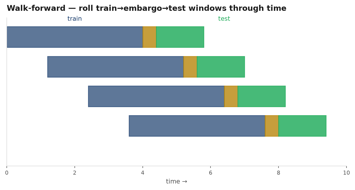
embargo \geq label horizon ⟹ no train outcome resolves inside the test block

A rolling walk-forward split with a purge-and-embargo gap between each train and test block — Purged, embargoed walk-forward: the gap between train and test must be at least the label horizon, or the label's own future leaks across the seam.

ek.ml.walk_forward_windows generates the rolling out-of-sample blocks with the purge and embargo built in; ek.ml.PurgedKFold does the same for hyperparameter selection inside a training window.

✦Scenario: the label that leaks 48 bars

Your triple barrier uses horizon_bars=48on M5 US100 — four trading hours. You split train/test at Friday's close. A candidate that fired at 15:40 Friday does not resolveuntil Monday, deep inside the test block — yet its features were computed Friday, so a naive split trains on a label whose outcome lives in the test period. The model has, in effect, read Monday's answer sheet. Purging drops that Friday candidate from training; a six-hour embargo (comfortably

\geq

the four-hour horizon) also drops the first few Monday candidates whose windows still overlap the seam. Skip this and your OOS AUC will look wonderful for a reason that has nothing to do with an edge — which is exactly what the label-shuffle test below is built to catch.

walk_forward.py

from edgekit.ml import walk_forward_windows, WalkForwardConfig

wf = WalkForwardConfig(train_days=7, test_hours=8, embargo_hours=6)   # embargo >= horizon
for w in walk_forward_windows(labels, wf):
    tr, te = labels.iloc[w["train_pos"]], labels.iloc[w["test_pos"]]
    m = make_model("hgb").fit(X.iloc[w["train_pos"]], tr["y"])
    proba = m.predict_proba(X.iloc[w["test_pos"]])       # honest OOS predictions
    # tune the take/skip threshold on an inner split of tr — never on te

!Tune the threshold on validation only

Choosing the

P \geq 0.55

cut-off (or any hyperparameter) on the same block you report results on is a leak. Use ek.ml.best_threshold on an inner validation split of the training window, then apply the frozen threshold on the test block unchanged.

The label-shuffle null test#

The single most useful sanity check for a meta-label: permute the labels, refit, and confirm the out-of-sample AUC collapses to ~0.5. If a model trained on shuffled labels still scores well, it is reading the future through a leak in your pipeline — the features or the split, not the market. Real signal dies under the shuffle; leakage survives it.

shuffle_label_gate(make_model_fn, X, y, r=None, n=10, test_frac=0.3, seed=0) -> dict
# returns {mean_auc, aucs, mean_ev} -- mean_auc should sit at ~0.5

shuffle_gate.py

from edgekit.ml import shuffle_label_gate, make_model
res = shuffle_label_gate(lambda: make_model("hgb"), X, y, n=10)
assert 0.45 < res["mean_auc"] < 0.55, "AUC on shuffled labels != 0.5 -> leakage in the pipeline"

Overfitting: the amplified risk#

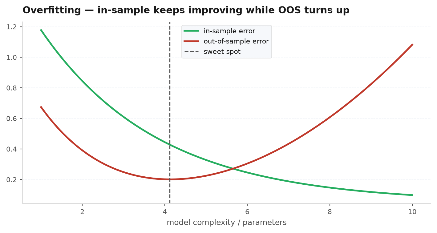
A hand-built rule has a handful of parameters; a gradient-boosted model has thousands of effective degrees of freedom. That flexibility is exactly what lets it memorise noise. Every overfitting lesson from overfitting detection applies here with the dial turned up: the more the model can fit, the more the in-sample score overstates the truth, and the wider the gap to out-of-sample.

Training score rising while validation score peaks and then falls as model complexity grows — The classic gap: as capacity grows, training score keeps climbing while true out-of-sample performance turns over. ML widens this gap faster than any rule.

!ML does not lower the bar — it raises it

Machine learning does not relax the validation gauntlet; it demands a stricter one. Report out-of-sample expectancy from purged walk-forward, pass the label-shuffle null, keep a sealed holdout you touch once, and prefer the simplest model that survives. A meta-label that only looks good in-sample is worth strictly less than the plain rule it sits on.

Cloud-safe tree export#

A trained model is useless if you can't run it where the strategy lives. ek.ml.export_trees serialises a fitted HistGradientBoostingClassifier to a plain string blob, and the pure-Python / pure-C# inference generated from it needs no scikit-learn at runtime — it drops into a cTrader cBot. The round-trip is guaranteed to float tolerance:

tree_predict_proba (blob, X) - clf.predict_proba (X) [:, 1] < 1 0^{- 6}

export.py

import numpy as np
from sklearn.ensemble import HistGradientBoostingClassifier
from edgekit.ml import export_trees, tree_predict_proba, emit_csharp

clf = HistGradientBoostingClassifier(max_depth=3, max_iter=40).fit(X, y)
blob = export_trees(clf)

# the guarantee: pure-python inference matches sklearn to 1e-6
assert np.abs(tree_predict_proba(blob, X) - clf.predict_proba(X)[:, 1]).max() < 1e-6

cs = emit_csharp({"orb": blob}, feature_names=feat_names)   # -> C# for a cTrader cBot

Next: one validated edge is rarely the end — Portfolio construction covers combining low-correlation books so the whole is steadier than any part.