Simulating markets

You have exactly one history — the single path the market happened to print. Every metric you compute is one draw from a distribution you never get to see. Simulation is how you widen the sample: generate price series the market could have printed, run the strategy on all of them, and ask whether the edge survives worlds that never happened. Used for validation it is a trap; used for robustness it is one of the sharpest tools you have.

Start from scratch with a coin. You flip it 100 times, count 58 heads, and wonder: is this a biased coin, or did a fair one just have a good run? You cannot answer from the single sequence in your hand — so you do the obvious thing and imagine flipping a fair coin 100 times, over and over, to see how often pure chance produces 58-or-more heads. A market history is exactly that one sequence of flips. Simulation is imagining the fair coin: build a world where you know there is no edge, run your strategy on thousands of draws from it, and see whether your backtest number is ordinary or extraordinary against that null. Everything in this chapter is that one move, dressed up for prices.

Why simulate at all#

A backtest answers “what would this strategy have done on the one path we observed?” That is a sample of size one. The realised Sharpe, the max drawdown, the worst losing streak — each is a point estimate with a confidence interval you cannot read off a single equity curve. Two honest ways to widen the sample:

• Resample the strategy's own trades — the bootstrap / Monte-Carlo of R-multiples covered in Monte Carlo. This reshuffles outcomes you actually observed.
• Resample the market itself — generate synthetic price paths from a model, then run the whole strategy on each. This is what this chapter is about. It stresses the entry/exit logic, not just the trade order, because on each synthetic path the strategy makes fresh decisions.

The random walk and geometric Brownian motion#

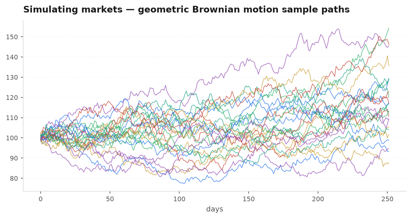
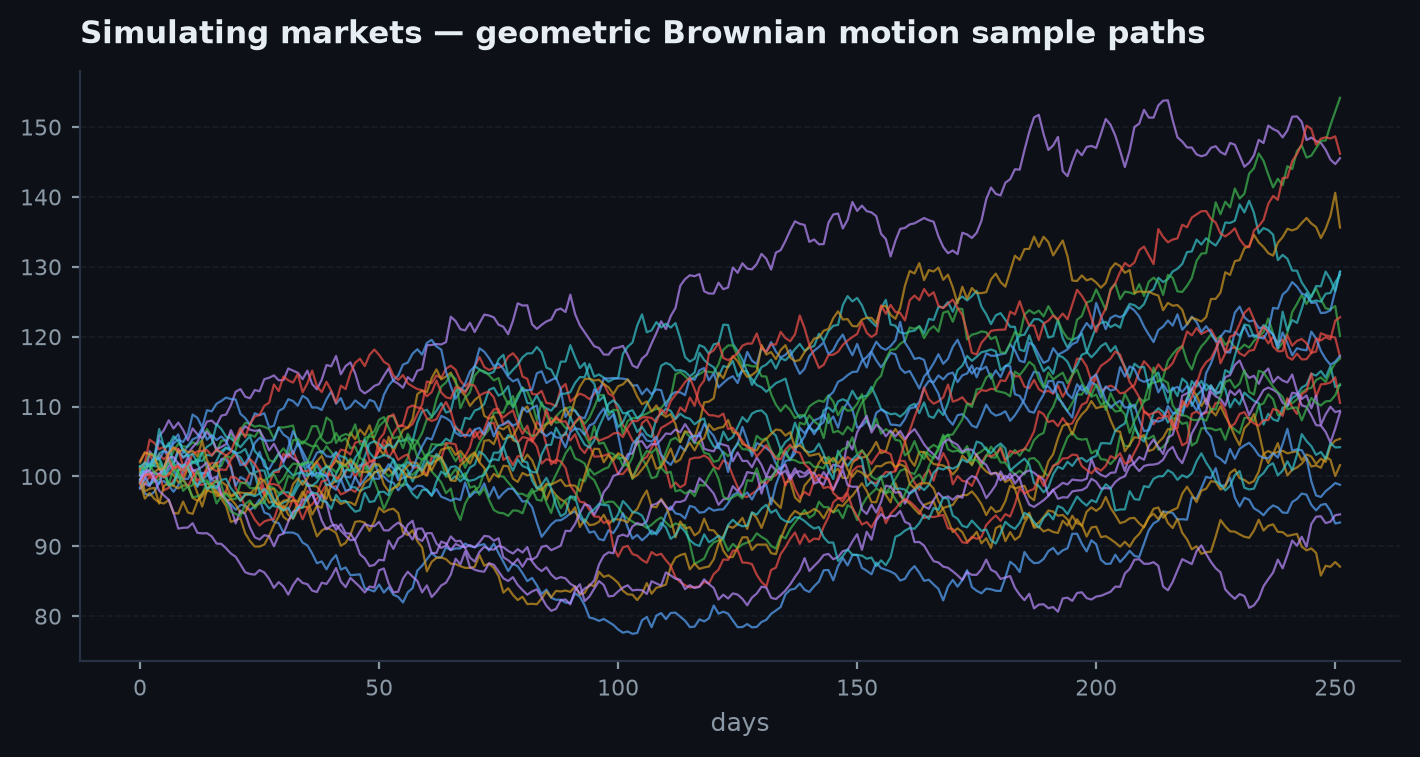
The textbook model of a price is a driftless-or-drifting random walk in log space. In continuous time it is geometric Brownian motion (GBM):

$S$ is the price, $\mu$ the drift, $\sigma$ the volatility, and $dW$ a Wiener increment. The reason GBM is the default is that it keeps prices positive and makes log-returns normal and i.i.d. To simulate it you discretise into a step of size $\Delta t$ and draw a standard-normal $z_t\sim N(0,1)$ each bar:

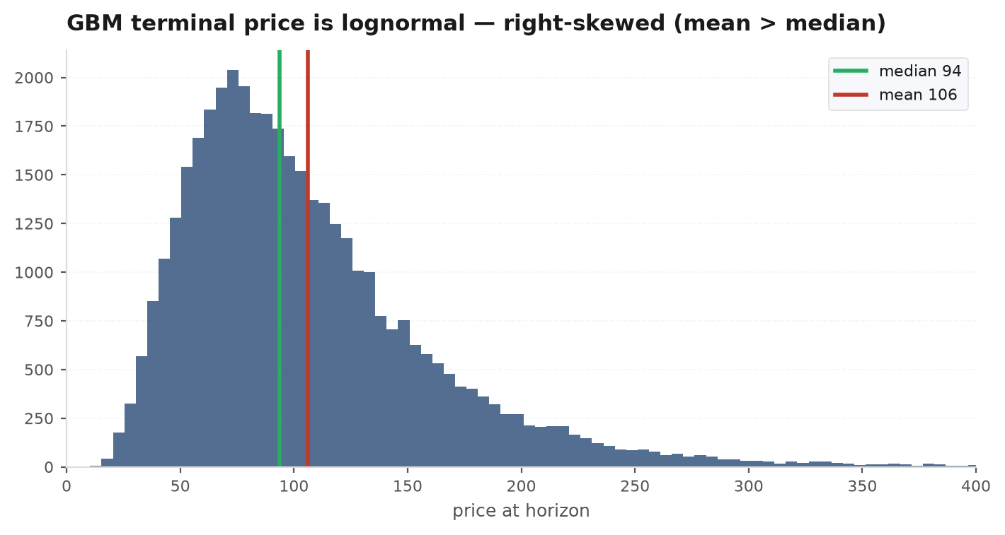
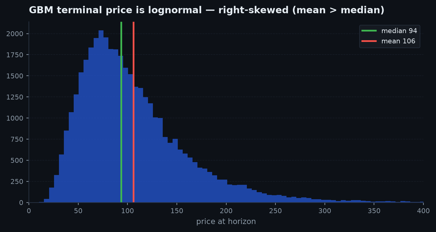
The $-\frac{1}{2}{\sigma }^2$ term is the Itô drift correction (the volatility drag from returns and compounding): without it the median path drifts up even at $\mu =0$. Setting $\mu =0$ gives a pure random walk — the null world in which no trend-following or mean-reversion rule should make money net of costs.

Generating paths and running a strategy on them#

edgekit strategies consume an OHLC frame, so the pattern is: simulate a close path, wrap it into a minimal bar frame, and call .backtest. Here a random walk ($\mu =0$) is fed to the illustrative SmaCross trend template — on a driftless series a trend rule should bleed the costs and nothing else, which is exactly the sanity check you want.

import numpy as np, pandas as pd
import edgekit as ek
from edgekit.strategy import SmaCross

def gbm_bars(n, mu=0.0, sigma=0.02, s0=100.0, seed=0):
    """One synthetic OHLC path from discretised GBM (dt = 1 bar)."""
    rng = np.random.default_rng(seed)
    z = rng.standard_normal(n)
    r = (mu - 0.5 * sigma**2) + sigma * z          # log-returns, dt = 1
    close = s0 * np.exp(np.cumsum(r))
    open_ = np.concatenate([[s0], close[:-1]])     # open = prior close
    wick = np.abs(rng.standard_normal(n)) * sigma * close
    idx = pd.date_range("2020-01-01", periods=n, freq="4h")
    return pd.DataFrame({
        "open": open_, "close": close,
        "high": np.maximum(open_, close) + wick,
        "low":  np.minimum(open_, close) - wick,
        "tick_volume": 1.0,
    }, index=idx)

# run the strategy on 500 independent null-world paths
finals = []
for seed in range(500):
    bars = gbm_bars(3000, mu=0.0, sigma=0.02, seed=seed)
    trades = SmaCross(fast=20, slow=100).backtest(bars, warmup=210, bars_per_day=6)
    finals.append(trades["r"].sum())              # terminal R on this path

finals = np.array(finals)
print(f"median terminal R = {np.median(finals):+.1f}   "
      f"P(profit) = {(finals > 0).mean():.0%}")

On a driftless random walk the distribution of terminal R should sit around a negative median once the default cost model bites, with $P(\text{profit})$ near a coin flip. If a rule looks strongly profitable on pure noise, the bug is in the backtest (look-ahead), not the market — see why backtests lie.

Adding jumps and fat tails#

Real returns are not Gaussian: they are fat-tailed and punctuated by jumps (gaps, flash crashes, headline moves). A GBM path drawn from a normal will systematically under-stress a strategy's stops and drawdowns. Two cheap upgrades:

• Student-t innovations — replace $z_t\sim N(0,1)$ with a (variance-rescaled) Student-t with low degrees of freedom $\nu$. Smaller $\nu$ = fatter tails; $\nu \to \infty$ recovers the normal.
• A jump-diffusion (Merton) term — add a compound-Poisson jump: with small per-bar probability $\lambda$ the return gets an extra shock $J\sim N({\mu }_J,{\sigma }_J^2)$.

def fat_tail_returns(n, sigma=0.02, nu=4, lam=0.01, jump_sd=0.10, seed=0):
    rng = np.random.default_rng(seed)
    t = rng.standard_t(nu, n) * np.sqrt((nu - 2) / nu)   # unit-variance t
    jumps = (rng.random(n) < lam) * rng.normal(0.0, jump_sd, n)
    return -0.5 * sigma**2 + sigma * t + jumps

Run the strategy across a sweep of $\nu$ and jump intensities and watch the max drawdown and worst-day statistics move. A rule whose survival depends on tails never appearing is not one you want sized to a hard drawdown budget (see prop-firm and capital).

Regime-switching simulation#

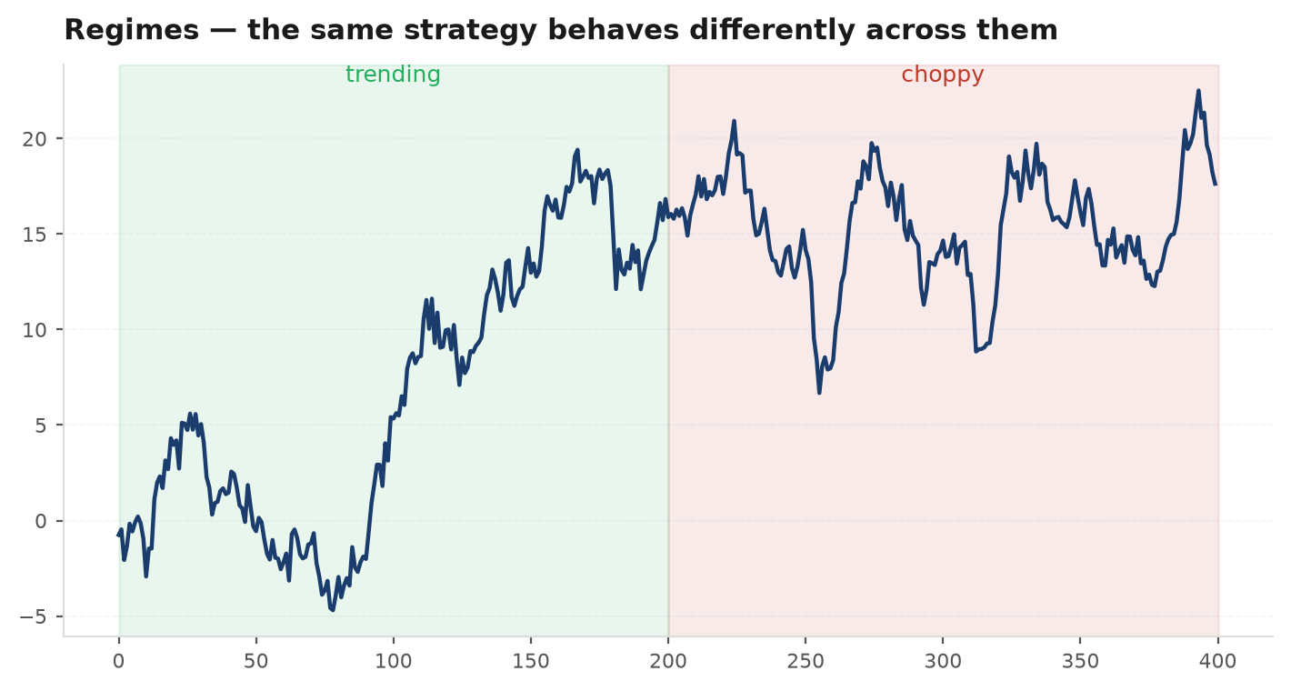
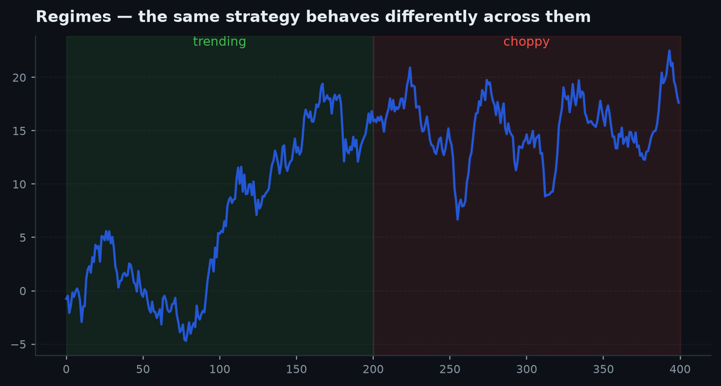
Markets are not stationary: they flip between calm and turbulent, trending and ranging. A single $(\mu ,\sigma )$ can never produce that. The simplest realistic generator is a two-state Markov chain — a low-vol trending regime and a high-vol choppy regime — with sticky transition probabilities so each state persists:

High $p_{00}$ and $p_{11}$ (say 0.98) make regimes last on average $1/(1-p)$ bars. This is the generator behind the classic test: a trend rule that prints beautifully in the trending state but gives it all back in the choppy state has a regime-dependent edge, and its live results will depend entirely on which regime it lands in.

def regime_returns(n, mus=(0.0008, -0.0002), sigmas=(0.008, 0.03),
                   p_stay=(0.98, 0.98), seed=0):
    rng = np.random.default_rng(seed)
    s = 0
    out = np.empty(n)
    for i in range(n):
        out[i] = rng.normal(mus[s], sigmas[s])
        if rng.random() > p_stay[s]:               # sticky switch
            s = 1 - s
    return out                                     # log-returns; exp-cumsum -> price

Stress-testing a strategy on synthetic series#

Put the pieces together into a stress harness: sweep a generator parameter, run the strategy on many seeds per setting, and summarise the R distribution with edgekit's metrics. The output is not “is this an edge” — it is “how does this rule degradeas the world gets meaner?”

import numpy as np
from edgekit import trade_stats

def stress(sigma, seeds=200):
    pfs = []
    for seed in range(seeds):
        bars = gbm_bars(3000, mu=0.0, sigma=sigma, seed=seed)
        tr = SmaCross(fast=20, slow=100).backtest(bars, warmup=210, bars_per_day=6)
        if len(tr):
            pfs.append(trade_stats(tr["r"].to_numpy())["pf"])
    return np.median(pfs)

for sigma in (0.01, 0.02, 0.04):
    print(f"sigma={sigma:.2f}  median PF over paths = {stress(sigma):.2f}")

At the desk. The sweep prints sigma=0.01 → PF 0.98, sigma=0.02 → PF 0.94, sigma=0.04 → PF 0.87. Read it as a slope, not three numbers: profit factor slides gently and monotonically as the world gets noisier, and every value sits just under 1.0 — precisely what a no-edge rule should do on a $\mu =0$ null. That is a healthy result: there is no hidden fragility that one particular vol setting detonates. Had a single setting jumped to PF 1.6 while its neighbours sat at 0.9, you would suspect the backtest was harvesting an artifact of that one generator — and you would go hunting for the look-ahead before trusting a live dollar to it.

The caveat, restated#

Synthetic markets are a lens for robustness, not a source of truth. They can tell you a strategy is fragile — a rule that dies the moment you add tails or flip regimes is telling you something real. They cannot tell you a strategy is good, because you built the world it succeeded in. Keep the two jobs separate: simulate to break things, validate on real out-of-sample data to believe things.

Next: from hand-written rules to learned ones — Machine learning in trading covers where ML actually helps (meta-labeling a rule, not predicting price) and the leakage traps that make most ML backtests fiction.