Entries, exits & stops

A signal tells you the market is interesting; the entry, the stop, and the exit decide whether that interest turns into R. This is where most of a strategy's realised behaviour is actually determined — and where a careless backtest manufactures phantom edge through optimistic fills. This chapter covers order types, gap-aware filling, stop placement, the exit families, and exactly how edgekit charges cost so your R-multiples are honest.

Order types#

Three primitives cover almost everything, and the choice trades certainty of fill against price:

• Market— fill now at whatever the next print is. Certain fill, uncertain price; you pay the spread and any slippage. This is what edgekit's research engine assumes: an EntryIntent is filled at the next bar's open.
• Limit — fill only at your price or better. Good price, uncertain fill: a limit into a pullback may never trigger, and the ones that do skip the trades that ran away without you (adverse selection).
• Stop — becomes a market order once price trades through a level. This is the breakout entry (buy-stop above the range) and the protective exit (sell-stop below the trade). Certain to trigger on a touch, but fills at the market beyond your level — worse in a gap.

Gap-aware fills — pessimism is the point#

The most seductive backtesting lie is assuming you got filled exactly at your intended price. Markets gap: overnight, over weekends, on news. If your breakout level is 100 and the bar opens at 103, you do not get 100 — you get 103. edgekit models this with two helpers the engine uses on every fill:

fill_entry(level: float, open_price: float, direction: int) -> float   # gap-aware entry fill
fill_stop(stop: float, open_price: float, direction: int) -> float     # pessimistic stop fill

• fill_entry — a long whose level gaps through fills at the higher open, never the stale level. You enter worse, so your R is smaller.
• fill_stop — a stop gapped through fills at the worseof the stop and the open. You exit worse, so a “−1R” stop can realise as −1.4R.

This is why the entry declares a level and a stop_dist, not a fill price: the strategy proposes, the engine fills — pessimistically — and reports the realised R.

Stop placement — the stop defines R#

The protective stop is not just risk control; its distance is the R denominator. Move the stop and you change what 1R means, which changes every downstream statistic. Two placements dominate:

ATR stop#

Set the stop a multiple of Average True Range away from entry, so risk is constant in volatility units rather than a fixed dollar/pip amount:

A wider ATR in a volatile regime gives a wider stop, so the same 1R absorbs the same amount of normal noise whether the market is calm or wild. This is what makes R comparable across regimes and instruments — and why the ATR stop is the default everywhere in edgekit. Use the lagged ATR:

from edgekit.core import lag
N = lag(ek.indicators.atr(bars.high, bars.low, bars.close, 20), 1)
# in entry(): EntryIntent(direction=1, level=level, stop_dist=2.0 * N[i])

Scenario (same trade, two regimes).You break long on BTCUSDT at 68,550 twice, months apart. In the calm regime ATR(20) is 700, so a 2-ATR stop is 1,400 points away at 67,150. In the volatile regime ATR(20) is 2,100, so the same 2-ATR stop sits 4,200 points away at 64,350. The dollar risk you assign is identical in both (1R), but the stop is three times wider when the market is wild — precisely so a normal volatile-regime wiggle doesn't masquerade as your idea being wrong. A fixed 1,000-point stop would have been noise-tight in the second case and got you swept before the move.

Opposite-edge (structural) stop#

Place the stop at a structural level — the other side of the range you broke out of, a swing low, the channel low. The ORB template does exactly this: the opening range's width is1R, so the stop sits at the opposite edge of the range. The advantage is that the stop is invalidation-based (“if price is back inside the range, the idea is wrong”) rather than an arbitrary distance.

Exits — where most of the character lives#

Two strategies with the same entry and stop can behave completely differently depending on how they leave. The exit shapes the entire right side of the R-distribution.

Protective stop#

The floor: the −1R backstop that is always active. Even when a strategy's exit returns None (hold), the engine keeps the stop live. Everything else is layered on top of this.

Fixed R-multiple target#

Flatten at a preset reward:risk. ORB(target_r=2.0) exits at $+2R$ (or session end). Targets cap the right tail — they raise the win rate but forgo the outsized winners, so they suit mean-reversion and range strategies more than trend-following. The relationship between the target multiple $b$ and the breakeven win rate is $p^{\ast }=1/(1+b)$: a 2R target only needs to win one time in three to break even (before cost).

Trailing stop#

Ratchet the stop toward price as the trade works — a Donchian/channel trail or a chandelier (high minus $k\cdot \text{ATR}$). This is the trend-follower's exit: it lets winners run open-endedly while continuously reducing give-back, which is what produces the fat positive tail. The cost is a lower win rate — many trades trail back to a small loss or breakeven.

def exit(self, bars, P, pos, i):
    # trailing channel exit for a long: leave when price closes back under the lagged lower channel
    if pos["dir"] == 1 and bars.close.iloc[i] < P["lo"][i]:
        return bars.close.iloc[i]
    return None    # otherwise hold; the protective stop still applies

Breakeven#

Once a trade reaches some profit (say $+1R$), move the stop to the entry price so the trade can no longer lose. It clips the left tail on trades that started well, at the cost of being stopped out of some that would have recovered after a normal pullback. Useful, but not free.

Time stop#

Exit after $m$bars regardless of price. A mean-reversion idea has a thesis with a clock — if the reversion has not happened in a few bars, it probably won't, and holding just accumulates risk. The time stop enforces that discipline and keeps capital turning over.

How edgekit charges cost — in R#

Cost is not a footnote; it is frequently the difference between a positive and negative edge, and it is charged directly in R so it shows up in every metric. The research engine subtracts a CostModelfrom each trade's R: by convention a round-trip fee plus a per-day holding (swap) charge. Because cost is denominated in the stop distance, a tighter stop pays a larger cost in R — a subtle, important effect that kills many high-frequency ideas.

Scenario (why the tight-stop scalper dies). Round-trip cost is a fixed 30 points on some CFD. The swing trader uses a 1,800-point ATR stop, so cost is $30/1,800=0.017R$ — a rounding error against a +1.5R winner. The scalper on the same instrument uses a 120-point stop; now the identical 30-point cost is $30/120=0.25R$ every trade. A scalper needs an expectancy above a quarter-R gross just to break even, and trades far more often. Same market, same fee schedule — the tight stop quietly multiplies the cost in R, which is how a gross edge that looks fine on paper nets to nothing.

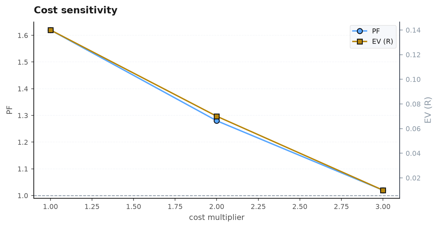
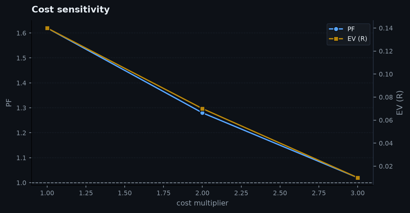
The practical consequence: always run a candidate at 2–3× your assumed cost. If the edge only exists at optimistic costs, it isn't one. edgekit's validation layer includes exactly this cost-stress; the bars_per_day argument you pass to .backtest is what converts a hold in bars into days for the swap charge (H4 = 6/day, a US cash minute session = 390/day).

Putting it together#

Entry fixes direction and the risk unit; the stop defines 1R and the left tail; the exit shapes the right tail; cost taxes all of it in R. Change any one and you get a different strategy, even with the same signal. Get in the habit of testing exit and stop choices as first-class variables — they are not tuning knobs to overfit, but they are where an idea becomes tradeable or not.

Next: Position sizing & risk — now that trades are priced in R, decide how many dollars ride on each one.