Anatomy of a strategy

Every mechanical strategy, however it dresses itself up, is four decisions bolted together: a signal that says when the market is interesting, an entry that commits capital, an exit that releases it, and a size that decides how much. This chapter takes that decomposition apart, ties it to the unit everything is measured in — the R-multiple — and shows the exact edgekit interface you implement to make it real.

The four decisions#

It is tempting to think of a strategy as “the indicator” — the moving-average crossover, the RSI threshold, the breakout level. But the indicator is only the signal. A tradeable strategy is the whole chain, and each link can make or break the edge independently:

• Signal — a condition on past data that flags a candidate: a close above a channel, an oscillator at an extreme, a spread stretched from its mean. It answers “is anything happening?”
• Entry — how and where you actually get in once the signal fires: at the next open, on a stop through a level, on a limit into a pullback. It also fixes the risk distance — the gap from entry to the stop that defines one unit of risk.
• Exit— the rules that end the trade: a protective stop, a profit target, a trailing channel, a time stop. Most of a strategy's character lives here, not in the entry.
• Sizing — how many dollars of risk ride on this particular trade. Sizing does not create edge, but it decides whether a real edge compounds or a run of losers ruins you.

The R-multiple is the unit#

edgekit prices every trade in R-multiples, not dollars or pips. One $R$ is the risk you committed on entry — the distance from your entry price to your initial stop. A trade that makes twice what it risked is $+2R$; one stopped out for its full risk is $-1R$ (a touch worse after cost). For a long,

where $d_{\text{stop}}$ is the stop distance in price units and $c$ is the round-trip cost, itself expressed in R. Working in R does three things at once. It makes trades on a $30 stock and a $60,000 coin directly comparable. It separates the edge (the R-distribution the strategy produces) from the sizing (how many dollars you assign per R) — the subject of a whole later chapter. And it lets the expectancy formula from the math of edge read straight off the trade list:

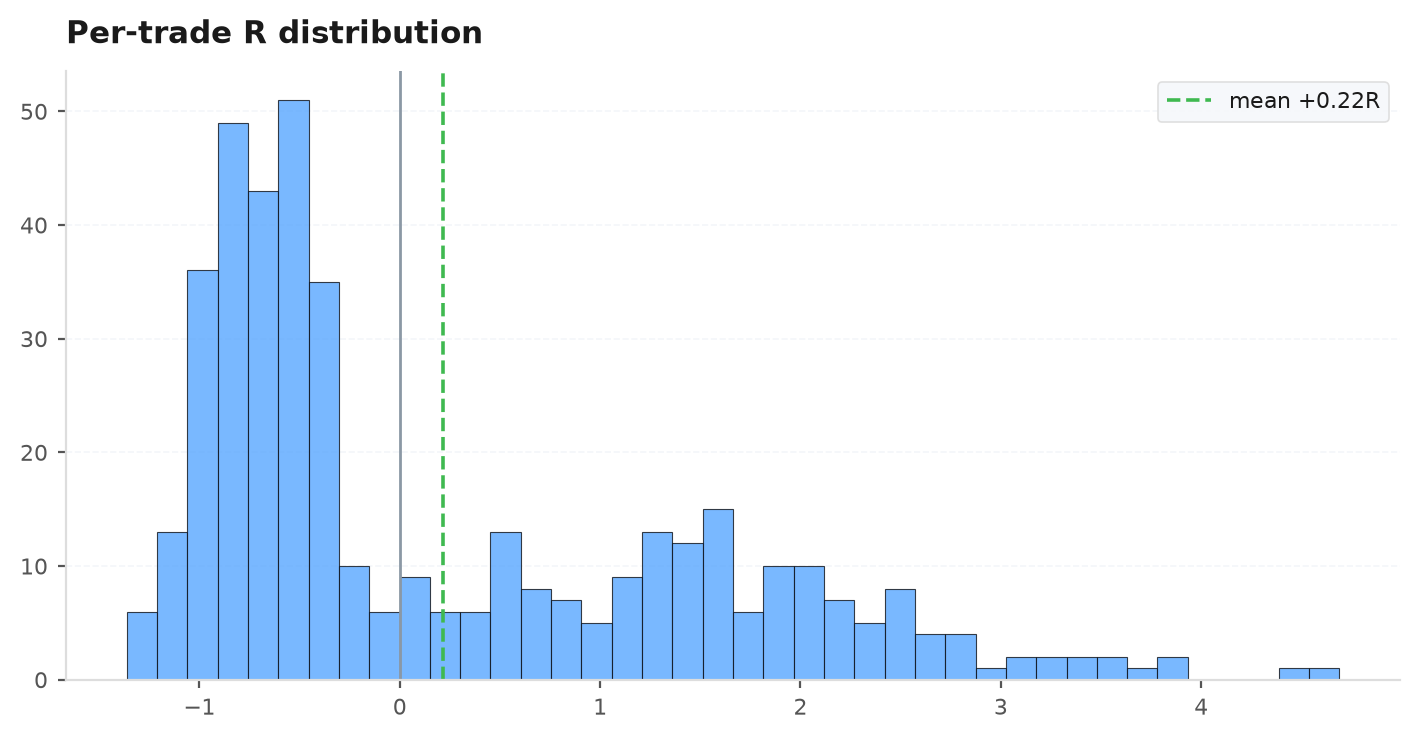
with $p$ the win rate, $W$ the average winner in R and $L$ the average loser in R. A strategy is worth trading only when $E[R]>0$ after costs — and a trend-follower can be profitable at a 40% win rate if $W$ is large enough, while a mean-reverter can win 70% of the time and still bleed if its losers are fat. The R-histogram is the picture of that distribution.

Scenario (reading R off a fill). Take the BTCUSDT trade above: entry 68,550, stop distance $d_{\text{stop}}=1,800$. The trail eventually fires and the engine closes it at 71,250. Ignoring cost, that is $(71,250-68,550)/1,800=+1.5R$. Charge a round-trip cost of, say, 0.05R and the booked trade is $+1.45R$. Had it instead gapped down and stopped, you would read roughly $-1R$ (a touch worse if the open gapped through the stop). Whether the coin trades at 68k or a stock trades at $30, that same +1.45 / −1.05 vocabulary lets you pool both onto one histogram and read the expectancy straight off the mean.

Causality: act on bar i using data through i−1#

The single rule that separates a real backtest from fiction: on bar $i$, a strategy may only use information that was actually knowable before bar $i$ traded. The close of bar $i$ is not known until bar $i$ is over, so a rule that decides at the open of $i$ must read indicators computed through $i-1$. Break this and the backtest quietly trades on the future — the most common way a “profitable” system turns out to be a mirage (see why backtests lie).

edgekit enforces causality structurally. Indicators in edgekit.indicators are deliberately un-lagged — index $i$ holds the value computed through bar $i$ inclusive — and it is your job to shift them by one bar with edgekit.core.lag before a rule acts on them. The engine then fills entries at the open of the next bar, gap-aware, so no trade is ever booked at a price the strategy could not have reached.

Scenario (the one-bar shift, concretely). Suppose bar $i$is the 08:00 UTC H4 candle on BTCUSDT and your rule is “go long on a break of the prior 20-bar high.” The naive code reads the Donchian upper channel at index $i$ — but that value already folds in bar $i$'s own high, which is not known until 12:00 when the candle closes. So the breakout is measured against a level that partly includes the very bar you are testing: guaranteed look-ahead. The lag fixes it — up_prev = lag(up, 1) means index $i$ now holds the channel through 04:00 (bar $i-1$), which is exactly what a trader staring at the chart at the 08:00 open could actually see. Same rule, honest data.

The edgekit Strategy interface#

A research strategy is a small class with a name and three methods — the runtime-checkable Strategy protocol that edgekit.engine consumes. Most strategies subclass BaseStrategy, which supplies the one-line .backtest wiring so you only implement the decisions:

prepare(self, bars) -> dict                        # precompute causal (lagged) indicator arrays — the P dict
entry(self, bars, P, i) -> EntryIntent | None      # entry decision on a FLAT bar i
exit(self, bars, P, pos, i) -> float | None        # exit price while IN a position on bar i

• prepare runs once at the start of a backtest. It computes every indicator the rules need and lags them, returning them in a plain dict conventionally called P.
• entry is called on each bar while flat. Return an EntryIntent to commit, or None to stand aside.
• exit is called on each bar while in a position pos. Return an exit price to close, or None to hold (the engine still enforces the stop).

EntryIntent — the entry as data#

The entry rule does not place an order directly; it returns an EntryIntent describing the trade, and the engine handles the (pessimistic, gap-aware) fill. Three fields:

EntryIntent(direction: int, level: float, stop_dist: float)

Note what is not here: no share count, no dollar amount. The research engine works entirely in R, so the entry only declares direction, where, and how far to the stop. Turning R into dollars is a separate, later decision handled by edgekit.sizing.

A minimal BaseStrategy skeleton#

Here is the whole pattern in one illustrative class — a plain channel breakout, shown for its structure, not as an edge to trade. Watch where the lag lives (in prepare) and how the entry expresses risk through stop_dist:

import edgekit as ek
from edgekit.strategy import BaseStrategy
from edgekit.engine import EntryIntent
from edgekit.core import lag

class ChannelBreakout(BaseStrategy):
    name = "channel_breakout"          # carried onto every trade's 'tag'

    def __init__(self, chan_n=20, atr_n=20, stop_mult=2.0):
        self.chan_n, self.atr_n, self.stop_mult = chan_n, atr_n, stop_mult

    def prepare(self, bars):
        up, lo = ek.indicators.donchian(bars.high, bars.low, self.chan_n)
        atr = ek.indicators.atr(bars.high, bars.low, bars.close, self.atr_n)
        # Lag EVERYTHING a rule will read on bar i — this is the causality contract.
        return {"up": lag(up, 1), "lo": lag(lo, 1), "atr": lag(atr, 1)}

    def entry(self, bars, P, i):
        level, atr = P["up"][i], P["atr"][i]
        if atr > 0 and bars.close.iloc[i] > level:      # break of the prior channel high
            return EntryIntent(direction=1, level=level, stop_dist=self.stop_mult * atr)
        return None                                     # otherwise stay flat

    def exit(self, bars, P, pos, i):
        # Illustrative trailing exit: leave when price closes back under the lower channel.
        if bars.close.iloc[i] < P["lo"][i]:
            return bars.close.iloc[i]
        return None                                     # else the engine's stop protects us

trades = ChannelBreakout().backtest(bars, warmup=210, bars_per_day=6)
print(trades["r"].sum(), len(trades))    # total net R, trade count

.backtest runs the class through the bar loop and returns the canonical trade frame — one row per closed trade, net R in the r column, exit date in date, plus dir, bars_held, entry, exit, stop_dist, and exit_reason. That frame is the raw material for every metric and every validation test that follows.

Where the pieces go from here#

The rest of Part III walks the four decisions one at a time. The next chapter builds the raw material for the signal — the indicator families and the lag discipline that keeps them honest. Then comes a taxonomy of the strategy archetypes those signals feed, a full worked build, the mechanics of entries and exits, and finally the math of sizing.

Next: Indicators & features — the vocabulary of signals, and the one lag rule that keeps them causal.