Position sizing & risk

Sizing does not create edge — a losing strategy sized any way still loses — but it decides whether a real edge compounds into wealth or gets wiped out by an unlucky run first. This chapter is the bridge from the R-multiples of the last five chapters to dollars: fixed-fractional risk, volatility targeting, Kelly and why you trade a fraction of it, and the drawdown-budget machinery edgekit uses to size a whole book to a hard risk limit.

Fixed-fractional risk#

The foundation: risk the same fraction $f$of current equity on every trade. Since a trade's risk is 1R (the stop distance), you convert R to dollars by choosing how many dollars 1R is worth:

with $E$ equity and $d_{\text{stop}}$ the stop distance in price units. Two properties matter. Because it scales with equity, wins compound and losses shrink the next bet — you can never (in theory) go fully bust on a series of −1R losses. And because risk is fixed per R, a volatile instrument with a wide ATR stop automatically gets fewer units, equalising risk across the book. A typical $f$ is 0.5–2% per trade; the ceiling is set by drawdown tolerance, below.

Scenario (R to contracts). Account $E=\$100,000$, risk $f=1\%$, so dollar risk is $1,000. Your BTCUSDT long has a stop distance of 1,800 points; at $1 per point per unit that is $1,000/1,800\approx 0.56$ BTC. Now the same account takes a low-vol trade with a 400-point stop: units become $1,000/400=2.5$ — over four times the size, because the tighter stop means each unit risks less. Both trades put exactly $1,000 at risk; the position size floats so the riskstays flat. Win the BTC trade at +2R and you make $2,000 (2%); lose it and you are down $1,000, and next trade's 1% is computed on the smaller $99,000 — losers automatically shrink the bet.

Volatility targeting#

Fixed-fractional holds per-trade risk constant; volatility targeting holds the portfolio's realised volatility constant. Scale exposure inversely to recent volatility so the book delivers a steady risk level instead of lurching with the market's mood:

When the book goes quiet the scale presses risk up; when volatility spikes it trims. edgekit's ek.sizing.vol_target implements exactly this, with two guardrails: the target is the book's own expanding median volatility (not a hand-picked number that invites overfitting), and the scale is clipped to $[0.5,\text{cap}]$ so it never de-levers below half or levers past the cap.

stable = ek.sizing.vol_target(book_r, cap=1.5)   # steady vol; scale clipped to [0.5, 1.5]

Scenario (leaning against the market's mood).Your book's own median trailing volatility is the target. Through a sleepy summer the book's realised vol drops to two-thirds of that median, so $\text{scale}={\sigma }_{\text{target}}/{\sigma }_t\approx 1.5$ — and the cap of 1.5 catches it exactly, pressing exposure up to fill the quiet. Then a volatility spike doubles realised vol; the scale wants to drop to ~0.5 and the floor clips it there, halving exposure so the book keeps delivering roughly the same risk instead of lurching with the tape. Without the clips a single freak-calm week could lever you to the moon right before the storm.

Kelly and fractional Kelly#

Kelly answers “what $f$maximises long-run compound growth?” For a bet paying $b$ to 1 with win probability $p$ (recall the math of edge):

Scenario (plug in a real backtest). Your validated trend-follower wins $p=0.42$ of the time and its average winner is 2.5× its average loser, so $b=2.5$. Then $f^{\ast }=(0.42\cdot 3.5-1)/2.5=0.19$ — full Kelly says risk 19% of equity per trade. That is terrifying: a run of four losers (entirely normal at a 42% win rate) would carve roughly 55% off the account. And your $p$ and $b$ came from a noisy backtest that almost certainly overstates the edge. Take half-Kelly and you risk ~9.5%; take the quarter-Kelly most desks actually run and you are near 4.75% — already aggressive, and a country mile below the raw number the formula spat out.

Betting more than $f^{\ast }$ lowers growth and raises risk — a strictly bad trade — and betting past $2f^{\ast }$ drives expected log-growth negative even with a positive edge. The growth-rate curve is a dome: it climbs to a peak at $f^{\ast }$ and falls away on the right.

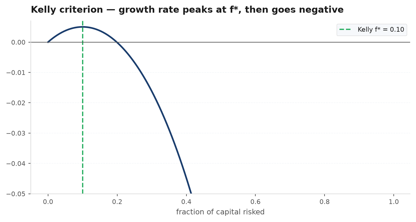
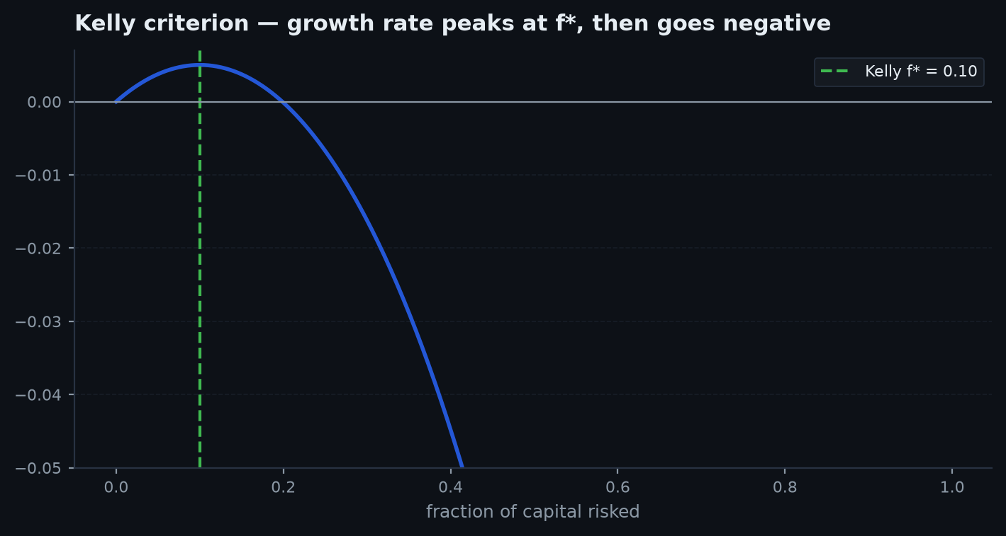
Nobody trades full Kelly. It assumes you know $p$ and $b$ exactly — you don't, you estimated them from a noisy backtest — and full Kelly produces drawdowns most humans cannot sit through. Overestimating the edge pushes you past the peak into the region where growth is negative. The standard defence is fractional Kelly: trade $\lambda f^{\ast }$ with $\lambda \approx 0.25\text{–}0.5$. Half-Kelly keeps about three-quarters of the growth for roughly half the volatility — a trade almost always worth making given estimation error.

Sizing to a drawdown budget#

In practice you rarely size from Kelly directly — you size to a drawdown limit, because that is the constraint that actually ends accounts (and the one prop firms enforce). The question inverts: given this strategy's R-stream and a maximum tolerable drawdown, how many dollars per R can I risk? edgekit answers it with ek.metrics.dd_matched_size — the single home for that math — wrapped by ek.sizing.size_to_dd, which returns the sized dollar series directly.

res = ek.sizing.size_to_dd(daily_r, dd_budget=0.095, account=100_000, daily_cap=0.045)
res["sized"]         # dollar P&L series; historical max DD == 9.5% of account (when max-dd binds)
res["dollar_per_r"]  # the dollars-per-R scalar this implies
res["binding"]       # "max-dd" or "daily" — which constraint set the size

Scenario (sizing to a prop limit).A $100k FTMO-style account allows a 10% overall drawdown; you budget 9.5% to leave a buffer. Your strategy's historical R-stream had a max drawdown of 22R. Then dollars per R = $(0.095\cdot 100,000)/22\approx \$432$: risk about $432 per trade and the historical path would have drawn down exactly to the 9.5% line at its worst. But add the daily_cap=0.045and if any single day's R-loss, scaled at $432/R, would breach 4.5% of the account, the daily rule binds first and res["binding"] returns "daily" — forcing a smaller size. Whichever leash is shorter is the one that sets your stake.

With a daily_cap, whichever constraint binds tighter wins — a dual limit that mirrors a prop-firm's combined max-drawdown and daily-loss rules (see prop-firm capital).

Risk of ruin#

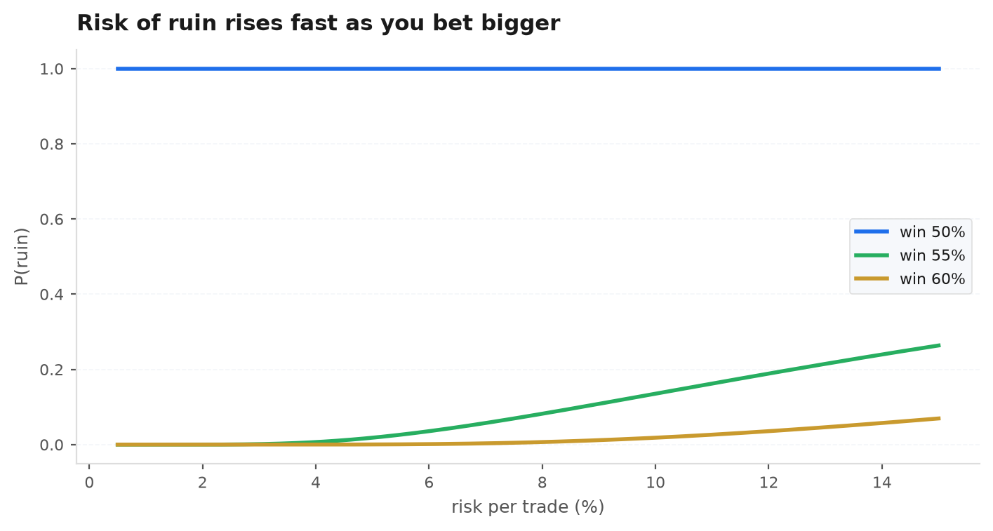
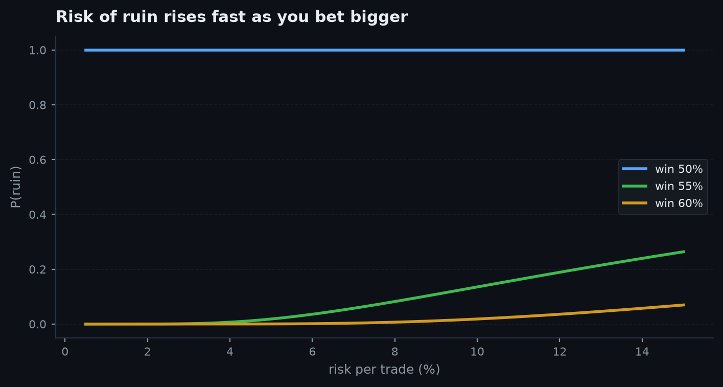
Why fractional matters, made quantitative. For a strategy with per-trade win probability $p$ risking a fraction that survives $N$ consecutive losses, the probability of eventually hitting a ruin threshold rises steeply as the bet fraction climbs. A useful closed form for even-money-style bets is

where $e$ is the edge and $u$ the number of risk-units of capital. The lesson is not the exact formula but its shape: ruin probability is exponentially sensitive to how much you risk per bet, so halving the bet fraction does far more than halve the tail risk.

Scenario (the convexity, concretely).Two traders share the same real edge but size it differently. Trader A risks 2% per trade, so a “ruin” drawdown is many risk-units of capital away — the probability of blowing up is a fraction of a percent. Trader B, sure the edge is bigger than it is, risks 8%. B has not merely quadrupled the risk: because $u$ (capital measured in risk-units) shrank by 4×, the ruin probability rose super-linearlyinto the double digits. Same signal, same win rate — one survives a bad streak, the other doesn't. Sizing didn't change the edge; it changed whether the trader is around to collect it.

Governing a book: risk parity, CPPI, drawdown throttle#

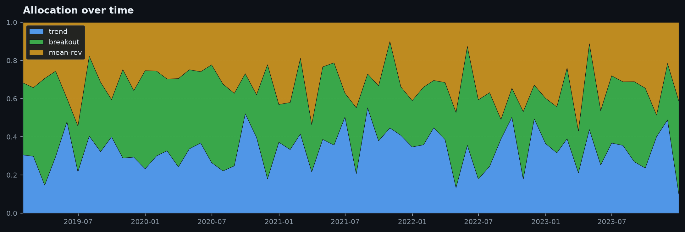
Once several validated strategies run together, sizing becomes allocation. edgekit separates three jobs:

Risk parity (inverse-vol)#

Weight each strategy by the reciprocal of its trailing volatility so no single loud asset dominates the book's risk — every sleeve contributes roughly equal risk rather than equal dollars:

w    = ek.sizing.risk_parity(M)        # M: columns are per-strategy daily-R series
book = (M * w).sum(axis=1)             # the equal-risk combined R-stream

CPPI — throttle up when winning, down when bleeding#

Constant-Proportion Portfolio Insurance runs a trailing floor below the high-water mark and risks in proportion to the cushion — the distance from equity down to that floor. Risk scales up while the book climbs and toward zero as it approaches the floor, which is the mechanism behind prop-challenge survival curves.

throttled = ek.sizing.cppi(daily_pnl, account=100_000, mstop=0.10, slope=2.0, cap=1.5)

Drawdown throttle#

The blunt version: halve risk whenever the equity curve is more than a threshold below its peak, restore it on recovery. Path-dependent and applied sequentially, it is a simple circuit-breaker on a live path.

out = ek.sizing.dd_throttle(daily_pnl, thresh=0.04, factor=0.5)   # halve risk while >4% underwater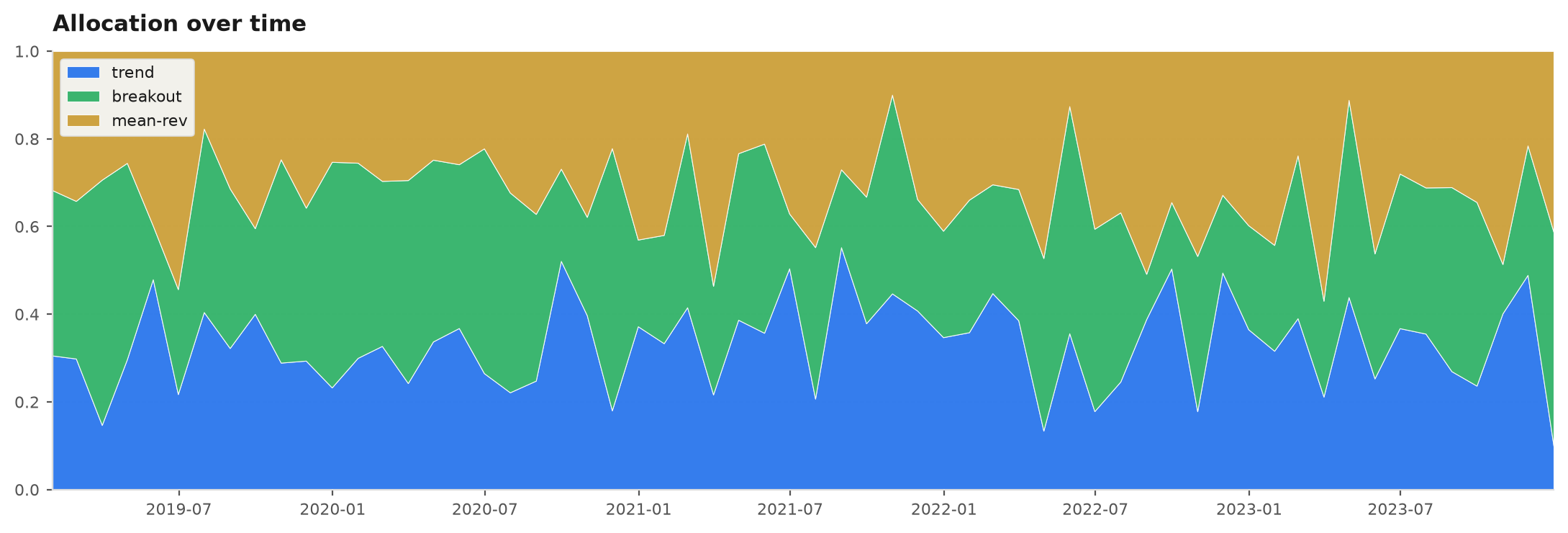

The order of operations#

Combine the sleeves (risk parity) → stabilise the book's volatility (vol-target) → size it to a drawdown budget in dollars (size-to-dd) → govern the live path (CPPI / throttle). Keeping these four steps separate is what lets you reason about each independently — and it is exactly how edgekit's sizing layer is factored. Sizing is the last thing you decide and the first thing that saves you.

Next: Part IV — Backtesting fundamentals, where we stop trusting a single equity curve and start proving whether the edge is real.