Indicators & features

Indicators are how a strategy compresses a stream of prices into a handful of numbers a rule can act on. There are only a few underlying ideas — level, direction, speed, spread, and dispersion — and almost every named indicator is one of them in disguise. This chapter walks the families, gives the one-line formula and the exact edgekit call for each, and nails down the causality rule that decides whether any of it means anything.

→An indicator is a feature, not a signal

On its own an indicator is just a transformed price series — a feature. It becomes a signal only when a rule reads it (“go long when the fast MA crosses the slow”). The same features also feed the machine-learning layer in Part V, where a model — not a hand-written threshold — decides what they mean.

The families#

Trend — where is the level, and which way is it drifting?#

Moving averages smooth price into a slow level so you can read direction. The simple moving average is the mean of the last $n$ closes; the exponential moving average weights recent bars more heavily and reacts faster:

SMA_{n} = \frac{1}{n} k = 0 \sum n - 1 P_{t - k}, EMA_{t} = α P_{t} + (1 - α) EMA_{t - 1}, α = \frac{2}{n + 1}

A rising average means the market is trending up on that horizon; the gap or crossover between a fast and a slow average is the classic trend signal. Longer $n$ = smoother but laggier.

ma_fast = ek.indicators.ema(bars.close, 20)
ma_slow = ek.indicators.sma(bars.close, 100)
ma200   = ek.indicators.sma(bars.close, 200)     # a common macro-trend gate: longs only above it

Scenario (a cross fires). On BTCUSDT H4, the fast EMA(20) has been sitting under the slow SMA(100) all through a two-week grind — no long allowed. On the 16:00 bar the EMA(20) prints 64,900 and the SMA(100) prints 64,700: the fast line has crossed above the slow one. At the desk that is the trend flag turning on. If price is also above the SMA(200) macro gate (say 61,000), a trend-follower now has permission to look for a long; if the fast line were still below the slow, the same bar would be ignored entirely.

Momentum — how fast, and is it overextended?#

Momentum oscillators measure the speed and one-sidedness of recent moves. The Relative Strength Index maps the ratio of average up-moves to average down-moves onto a bounded 0–100 scale:

RSI = 100 - \frac{100}{1 + R S}, R S = \frac{avg gain _{n}}{avg loss _{n}}

High RSI flags an overbought push, low RSI an oversold washout. A trend-follower reads a high RSI as strength; a mean-reverter reads the same value as a fade candidate — the indicator is neutral, the interpretation is the strategy. The fast $n = 2$ variant is the short-horizon exhaustion flag; longer $n = 14$ is the smoother momentum read.

rsi_fast = ek.indicators.rsi(bars.close, 2)      # short-term exhaustion
rsi      = ek.indicators.rsi(bars.close, 14)     # smoother momentum

Scenario (same number, two strategies).ETHUSDT has run hard and the RSI(14) reads 78. A trend-follower sees 78 and thinks “strength — the move has thrust, stay long.” A mean-reverter sees the identical 78 and thinks “overbought — fade it back toward the mean.” The oscillator has not taken a side; the strategy has. That is why the RSI belongs to the feature layer, not the signal — the same column feeds opposite trades depending on which archetype reads it.

Volatility — how big is a normal move right now?#

Volatility indicators size the market's current wiggle so risk can be set relative to it. Average True Range is the mean of the true range — the largest of today's high−low and the gaps to the prior close:

T R_{t} = max (H_{t} - L_{t}, ∣ H_{t} - C_{t - 1} ∣, ∣ L_{t} - C_{t - 1} ∣), ATR_{n} = mean_{n} (T R)

ATR is the workhorse behind the R-multiple: a stop set at $k \times ATR$ keeps the risk-per-trade constant in volatility units across calm and wild regimes, which is what makes R comparable through time. The log-space variant normalises range so it is comparable across price levels, and the Average Directional Index turns range into a trend-strength score (low ADX = chop, a natural gate to sit out).

atr    = ek.indicators.atr(bars.high, bars.low, bars.close, 20)     # stop distance / R unit
atr_lg = ek.indicators.atr_log(bars.high, bars.low, bars.close, 84) # regime-comparable vol
adx    = ek.indicators.adx(bars.high, bars.low, bars.close, 14)     # trend strength (gate chop)

Scenario (ATR sets the risk, not the price).In a calm July stretch BTCUSDT's H4 ATR(20) is 700 points; after a macro shock it jumps to 2,100. A fixed 1,000-point stop would be three noise-bars wide in calm and get tapped on the first wiggle in stress. A $2 \times ATR$ stop instead sits 1,400 points away in calm and 4,200 in stress — so “one R” always means the same amount of normal movement. That is the whole trick behind volatility-normalised risk: the dollar stop moves so the R stays constant.

Channels — has price left its recent envelope?#

A channel wraps price in a band; a break of the band is the event. The Donchian channel is the simplest — the highest high and lowest low of the last $n$ bars — and is the engine behind breakout systems. Keltner-style envelopes instead centre on a moving average and widen by a multiple of ATR:

upper_{n} = k < n max H_{t - k}, lower_{n} = k < n min L_{t - k}; EMA_{n} \pm m \cdot ATR_{n}

A close above the upper band is a “price is escaping its range” signal; the opposite band or the centre line is a natural exit. edgekit ships the Donchian primitive; the ATR-envelope you build from ema + atr.

up, lo = ek.indicators.donchian(bars.high, bars.low, 20)   # breakout channel
mid    = ek.indicators.ema(bars.close, 20)
band   = mid + 2.0 * ek.indicators.atr(bars.high, bars.low, bars.close, 20)

Scenario (the band is the event). The 20-bar Donchian upper on BTCUSDT H4 has been flat at 66,900 for days while price coils beneath it. The 20:00 bar closes at 67,300 — price has escaped the top of its three-day envelope. That single event is the breakout signal; the lower band at 63,100 is the natural opposite-edge stop, so the channel hands you both the trigger and the risk in one primitive.

Mean-reversion — how far from fair is price?#

Mean-reversion features measure distance from a referencein standard-deviation units, so “far” is defined statistically rather than by eyeballing. The rolling z-score is the canonical one:

z_{t} = \frac{x _{t} - μ _{n} ( x )}{σ _{n} ( x )}

where $μ_{n}$ and $σ_{n}$ are the trailing mean and standard deviation over $n$ bars. A large positive $z$ says price is stretched high relative to its recent range — a fade candidate if the series actually reverts. The same z-score is the core of a stat-arb spread signal, applied to the residual of one asset regressed on another rather than to raw price.

z = ek.indicators.zscore(bars.close, 60)   # standardised distance from the trailing mean

Scenario (how far is “far”?).A stock's 60-bar mean is $148 with a standard deviation of $2. Today it prints $153 — a big-looking $5 pop, but that is $z = + 2.5$ , genuinely stretched. Now a different, jumpier name has a 60-bar mean of $148 and a standard deviation of $6; the same $153 print is only $z = + 0.8$ — barely a ripple. The z-score converts “how many dollars” into “how many typical bars,” which is the only version of “far” a fade should act on — and only if the series actually reverts, which the next chapter tests.

The causality rule: lag every feature#

Here is the rule that everything hinges on, and the one most retail backtests get wrong. Every indicator in edgekit is returned un-lagged. Index position $i$ holds the value computed through bar $i$ inclusive — a number you only truly know once bar $i$ has closed. A rule that reads it while deciding what to do on bar $i$ is peeking at the current, completed bar. The fix is a one-bar shift with edgekit.core.lag:

causality.py

import edgekit as ek
from edgekit.core import lag

# WRONG — reads bar i's own completed ATR while acting on bar i (look-ahead)
N_bad = ek.indicators.atr(bars.high, bars.low, bars.close, 20)

# RIGHT — lag by one bar so N[i] reflects only what was known at the close of i-1
N     = lag(ek.indicators.atr(bars.high, bars.low, bars.close, 20), 1)
up, _ = ek.indicators.donchian(bars.high, bars.low, 20)
up_prev = lag(up, 1)          # a breakout on bar i is measured against the PRIOR channel

edgekit keeps the lag at the call site on purpose. Baking a shift into each indicator would hide the single most consequential modelling decision you make; leaving it explicit means every strategy's prepare method visibly declares which bar of information it acts on. The habit costs one function call and buys you a backtest that is not lying to you.

Scenario (a one-line leak worth 20% a year).A researcher backtests “buy when the RSI(2) crosses up through 10” on ETHUSDT and gets a dazzling curve. The bug: the un-lagged RSI at bar $i$ is computed through bar $i$ 's close, so the rule is really buying bars that already closed with a low RSI — it is peeking at the close it claims to act before. Add lag(..., 1) and the entry now keys off the RSI known at the prior close; the curve loses most of its gain. Nothing about the idea changed — only whether the backtest was allowed to see the future.

✕Look-ahead is the number-one way backtests inflate

Reading an un-lagged indicator, resampling with right-labelled bars, or computing a rolling stat over the full sample all leak the future into the past. The result is a gorgeous equity curve that evaporates live. Part IV's why backtests lie catalogues the whole family; the lag is your first line of defence against it.

Features track regimes — which is the point and the trap#

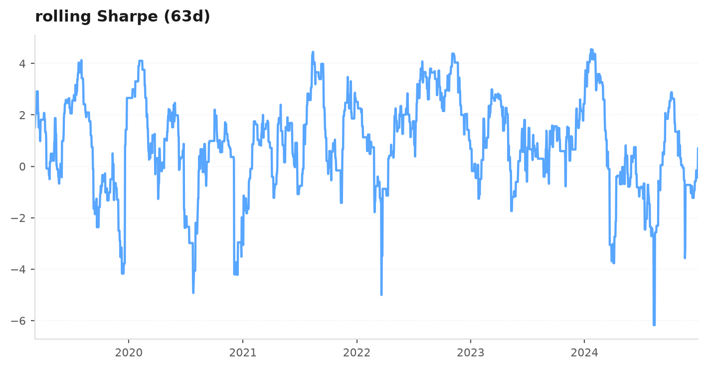
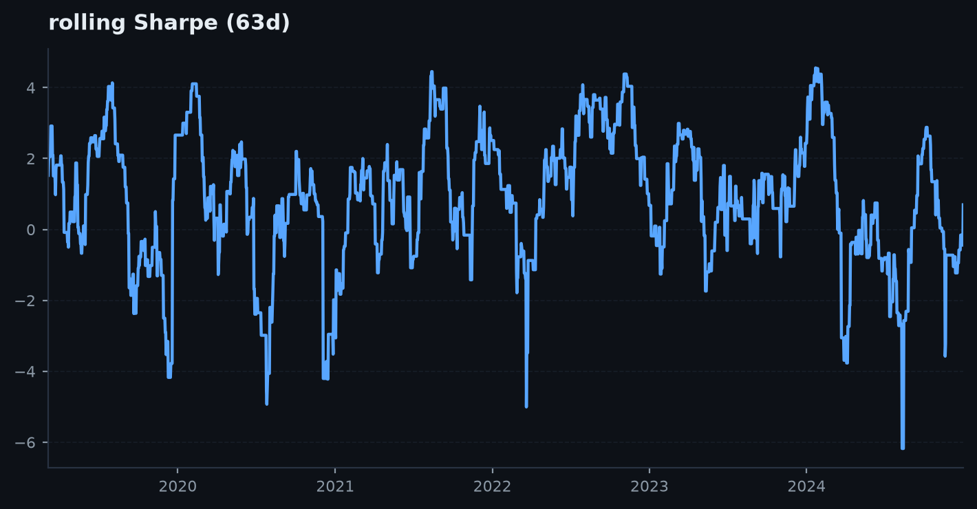
A good feature is informative precisely because it moves as the market's regime moves: ATR expands in stress, ADX rises in trends, z-scores blow out in dislocations. That responsiveness is what a rule exploits — and also why a single fixed threshold rarely holds across regimes. Volatility-normalised features (anything divided by ATR) travel across regimes better than raw-price ones, which is why R-multiples and ATR stops recur everywhere in edgekit.

Rolling indicator statistics over time — Features are not static: a rolling statistic drifts with the regime. Normalising by volatility is what keeps a threshold meaningful across calm and stressed periods.

From feature to strategy#

Everything here plugs into the prepare method from the previous chapter: compute the features you need, lag them, stash them in the P dict, and let entry/exit read them by index. What differs between a trend-follower, a breakout, and a mean-reverter is not the indicator library — it is which features they read and which direction they trade the reading. That is the map the next chapter draws.

Next: A taxonomy of strategies — the archetypes these features feed, what each one exploits, and when it fails.