Build your first strategy
Enough theory — let's run something. This chapter takes two shipped templates, SmaCross (a swing trend-follower) and ORB (an intraday breakout), from raw bars to a trade list to honest statistics. The point is not to discover an edge — neither of these is one as-is — but to learn the loop you will repeat for every real candidate: load, shape, backtest, read the numbers.
Step 1 — load and shape the data#
Everything starts with a clean OHLC frame. ek.data.load_bars reads a HistoryExporter CSV or a processed parquet split, validates the schema, and returns a monotone, de-duplicated frame indexed by UTC time. A swing strategy then wants a coarser timeframe, so we resample the fine bars up with ek.data.resample_ohlcv — which does the only correct aggregation (first open, max high, min low, last close, summed volume) and keeps the causal label="left" convention.
import edgekit as ek

bars = ek.data.load_bars("BTCUSDT_5m.csv")     # 5-minute bars, DatetimeIndex(UTC)
h4   = ek.data.resample_ohlcv(bars, "H4")      # up to 4-hour swing bars

print(ek.data.integrity_report(bars, bar_minutes=5)["intraweek_gaps"]) # inspect before trustingek.data.integrity_reportfirst. Silent gaps, zero-range bars, or spikes will quietly distort a backtest; knowing the data's real span and holes is step zero, not an afterthought.Step 2 — run the SmaCross backtest#
SmaCross goes long/short on a fast-vs-slow moving-average relationship, with an ATR-based stop that sets the R denominator. Constructing it and calling .backtest runs the full causal bar loop and hands back the canonical trade frame. bars_per_day=6 tells the engine an H4 day is six bars (for the time-based swap cost).
from edgekit.strategy import SmaCross

strat  = SmaCross(fast=20, slow=100, atr_n=20, stop_mult=2.0)
trades = strat.backtest(h4, warmup=210, bars_per_day=6)

trades.head()          # one row per closed trade, net R in the 'r' column
The trade frame is the same shape for every research strategy. The columns you will actually read:
| Column | Meaning |
|---|---|
r | Net R-multiple of the trade (after costs) — the number everything is judged on. |
date | Exit timestamp — used to annualise and to build the daily-R stream. |
dir | +1 long / −1 short. |
bars_held | Holding period in bars. |
entry, exit | Fill prices. |
stop_dist | The stop distance that defined 1R for this trade. |
exit_reason | Why the trade closed — stop, target, trailing exit, session end. |
Step 3 — read the statistics#
A trade list is not a verdict; ek.trade_stats turns it into one. Feed it the R column, and pass the exit dates to unlock the annualised and drawdown metrics.
st = ek.trade_stats(trades["r"], dates=trades["date"])

print(st["n"], st["ev_r"], st["win_rate"])     # count, expectancy per trade (R), hit rate
print(st["pf"], st["mar"], st["ann_r"])        # profit factor, return/maxDD, annualised R
print(st["max_dd_r"], st["worst_day_r"])       # the pain: worst drawdown and worst day, in R
The number that decides everything is expectancy, , reported as ev_r. A positive ev_r that survives costs is the necessary (not sufficient) condition for an edge. Judge the whole picture on pf (profit factor) and mar (return over max drawdown) rather than Sharpe alone — Sharpe systematically understates a skewed trend-following return, as edgekit.metrics warns.
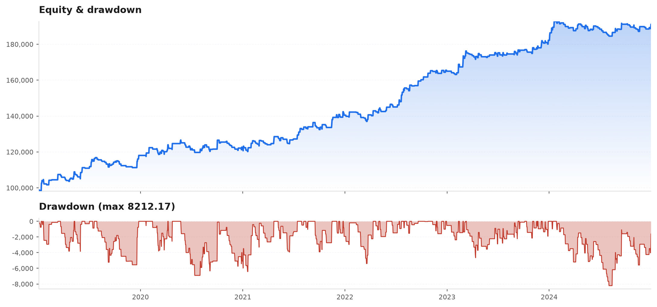
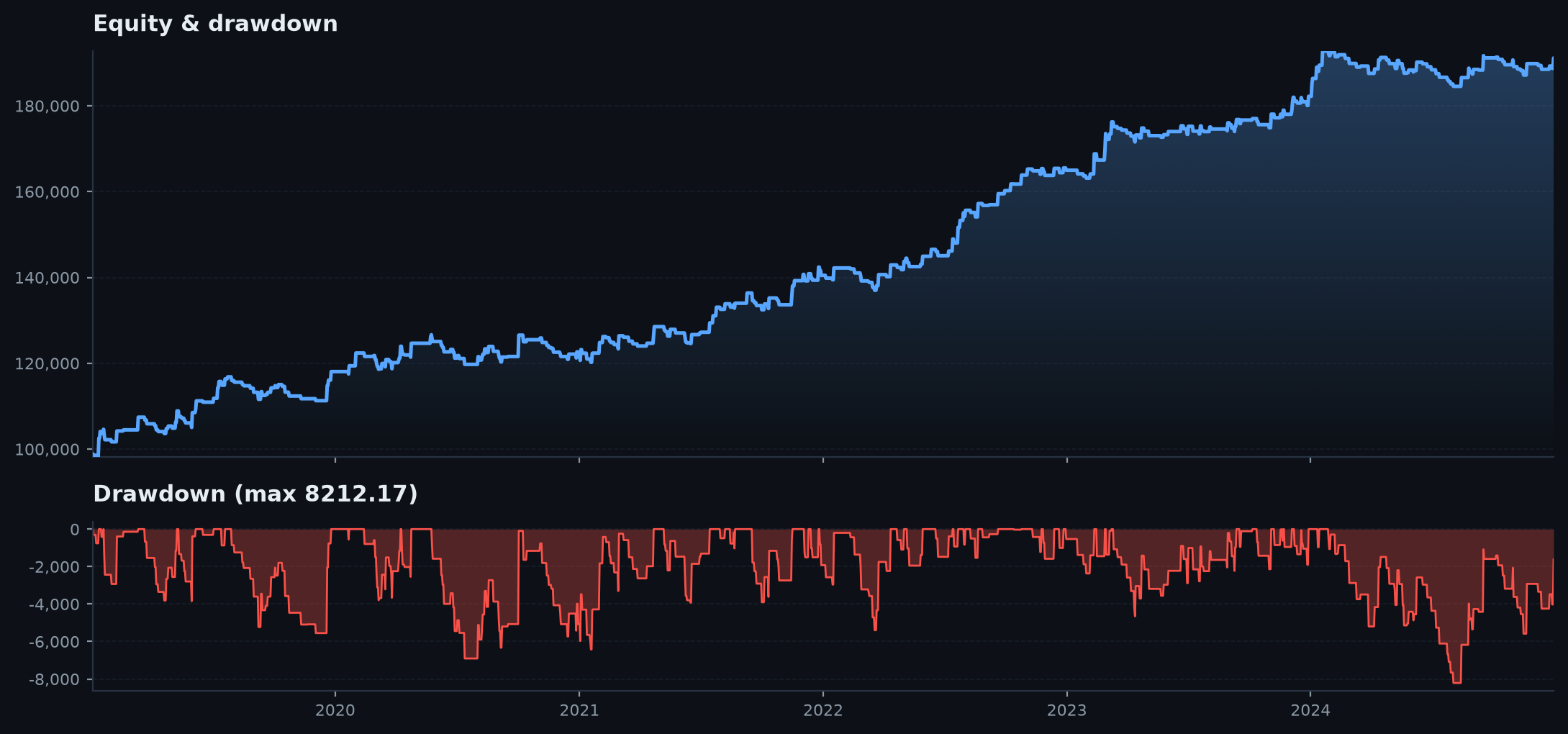
Say the run above comes back with n=143, ev_r=0.04, win_rate=0.41, pf=1.08, mar=0.6, max_dd_r=14.2. Walk it: 143 trades is enough to have an opinion. Expectancy is +0.04R per trade — barely positive, and a realistic cost bump could erase it. The 41% win rate confirms this is behaving like a trend-follower (most trades lose small). Profit factor 1.08 means you made $1.08 gross for every $1.00 lost — thin. And max_dd_rof 14.2 says that at some point you were fourteen full risk-units underwater: at 1% risk per trade, a ~14% equity drawdown you had to sit through to collect that 0.04R edge. That is the honest verdict — not “it works,” but “there might be something here, and it is not yet worth trading.”
Step 4 — the intraday ORB, and why session-slicing matters#
ORB is a different animal: an intraday opening-range breakout that needs a session, not a continuous stream. Each trading day's first or_bars bars define a range whose width is 1R; a break of the high goes long, of the low short, stop at the opposite edge, one trade per day. So the frame must be sliced to a trading session first — here US cash hours in New York — via ek.data.rth_mask, and the engine told the intraday bar count.
from edgekit.strategy import ORB

m1  = ek.data.load_bars("US100_M1.csv")        # 1-minute index bars
rth = m1[ek.data.rth_mask(m1.index, start="09:30", end="16:00", tz="America/New_York")]

orb    = ORB(or_bars=30, target_r=2.0)         # 30-min opening range, flatten at 2R
trades = orb.backtest(rth, warmup=5, bars_per_day=390)

st = ek.trade_stats(trades["r"], dates=trades["date"])
print(st["n"], st["ev_r"], st["pf"]) # well-powered trade count; expectancy near zeroORBderives its opening range from each bar's calendar day, so localise and mask the frame to your session first. Being intraday, it takes a small warmup and a bars_per_day matching your bar size (390 one-minute bars in a US cash session). The raw breakout is typically net-negative — the published edge comes from a walk-forward ML meta-label layered on top, not from this skeleton.Scenario (one ORB day). Take 2024-02-13 on US100. The 09:30–10:00 opening range spans 17,960–18,004 — a 44-point range, so 1R = 44 points and the target sits 88 points past the break. At 10:12 a one-minute bar pokes above 18,004, the engine fills the long at the next open (18,007, a few ticks of slippage past the level), stop at 17,960. Price drifts up to 18,050 then rolls over and tags the stop at 15:40 for . Repeat that across ~250 trading days a year and you get the hundreds of trades below — most days a small win or loss, no single day decisive. That volume is the point.
With hundreds of trades, ORB is well-powered: you can actually measure its expectancy rather than guess. A well-powered result of “roughly zero after cost” is far more useful than a spectacular number from nine trades — it tells you the raw signal has no edge, cleanly, so any effort goes into the selection layer.
Step 5 — look at the distribution, not just the mean#
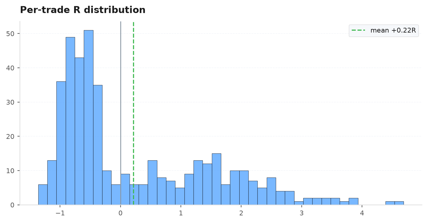
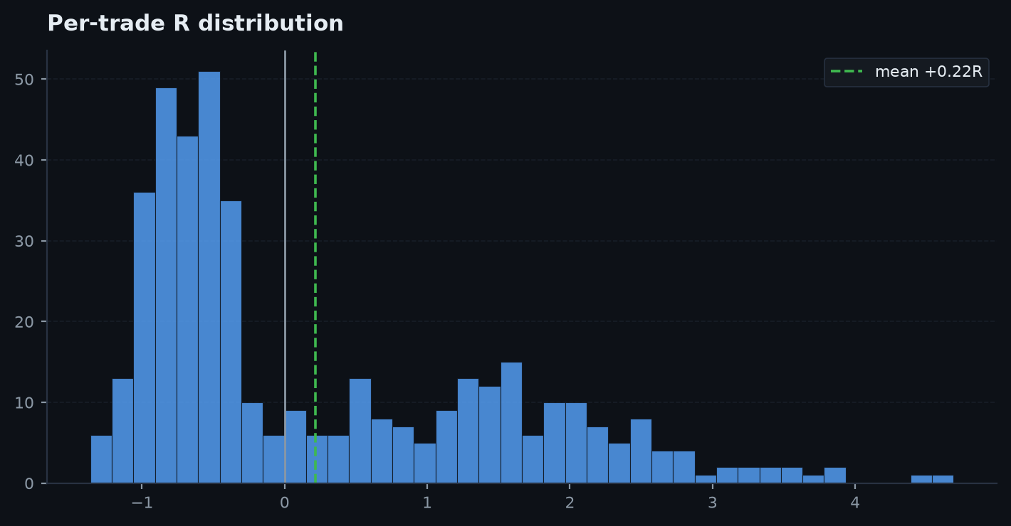
Two strategies with identical expectancy can be wildly different to trade. Plot the R-histogram to see the shape: a trend-follower shows many small losers and a few large winners (positive skew); a mean-reverter shows the mirror. The mean is the edge, but the tails are what you have to live through.
The loop you just learned#
Load → shape → backtest → read the stats → look at the distribution. That five-step loop is the entire inner cycle of strategy work; everything else is doing it more carefully. Two habits from this chapter carry forward: always report expectancy and profit factor (not hit rate or Sharpe alone), and always distrust a great number that rests on few trades.
A single backtest number is still just one draw, though — the next two chapters sharpen the machinery (entries, exits, sizing) and then Part IV asks the real question: is any of this actually significant?
Next: Entries, exits & stops — the order mechanics and exit rules that shape the R-distribution you just plotted.