Time-series analysis for OHLC

Before you fit a rule to a price series, you owe it one honest question: what kind of series is this? A trend model on a random walk and a reversion model on a runaway trend both lose money for the same reason — a mismatch between the strategy's assumption and the data's actual memory structure. This chapter is the toolkit for reading that structure: stationarity, the trend-vs-reversion tests, autocorrelation, volatility clustering, and seasonality — each with the exact edgekit.timeseries call.

→Run stats on returns, not prices

Almost every statistic in this chapter assumes the series is stationary — its mean, variance, and autocorrelation don't drift over time. A raw price series is not stationary, so you transform it first (log returns, or differencing) and analyse the transformed series. The one exception is the random-walk tests themselves (variance ratio, ADF), which take the level series precisely to ask whether it has a trend.

Why stationarity matters#

A stationary series is one whose statistical fingerprint stays put: the mean you estimate on the first half is the mean you'll see in the second half, the variance is stable, and the correlation between two points depends only on the gap between them, not on where they sit in time. That is the assumption baked into nearly every estimator — a rolling mean, a z-score, a regression coefficient — because each one pools information across time as if the underlying process weren't moving under your feet.

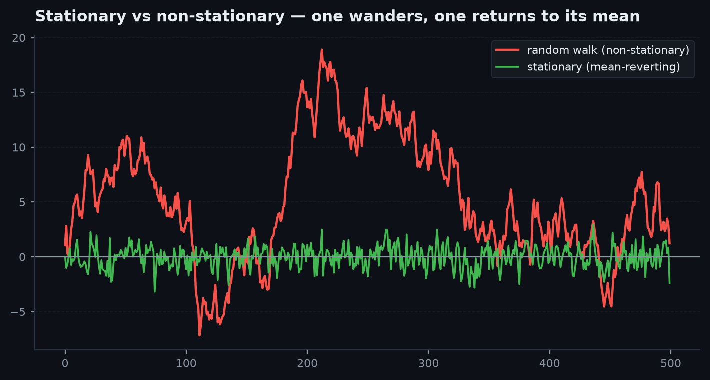
A price series breaks that assumption in the most fundamental way. The canonical model of a price is a random walk: each price is the last price plus an unpredictable shock.

P_{t} = P_{t - 1} + ε_{t}, ε_{t} \sim iid (0, σ^{2})

The variance of $P_{t}$ grows without bound as $t$ increases (it is $t σ^{2}$ ), so there is no fixed mean to revert to and no stable variance to standardise by. Compute a z-score of a random walk and the “distance from the mean” you get is meaningless, because the mean itself is wandering. This is why a strategy fit to price levels so often looks brilliant in-sample and dies out-of-sample: it learned the sample's particular wander, not a repeatable relationship.

The fix is to stationarise. Differencing the series once removes the stochastic trend, and for prices the natural first difference is the log return:

r_{t} = lo g P_{t} - lo g P_{t - 1} = Δ lo g P_{t}

Returns hover around a stable mean of roughly zero with a (mostly) stable variance — a series statistics can actually work on. In edgekit that transform is one call, and the differencing primitive is there for higher orders or non-price series:

import edgekit as ek

rets = ek.timeseries.log_returns(bars.close)   # stationarise prices -> returns
diff = ek.timeseries.difference(some_series, d=1)  # general d-th order difference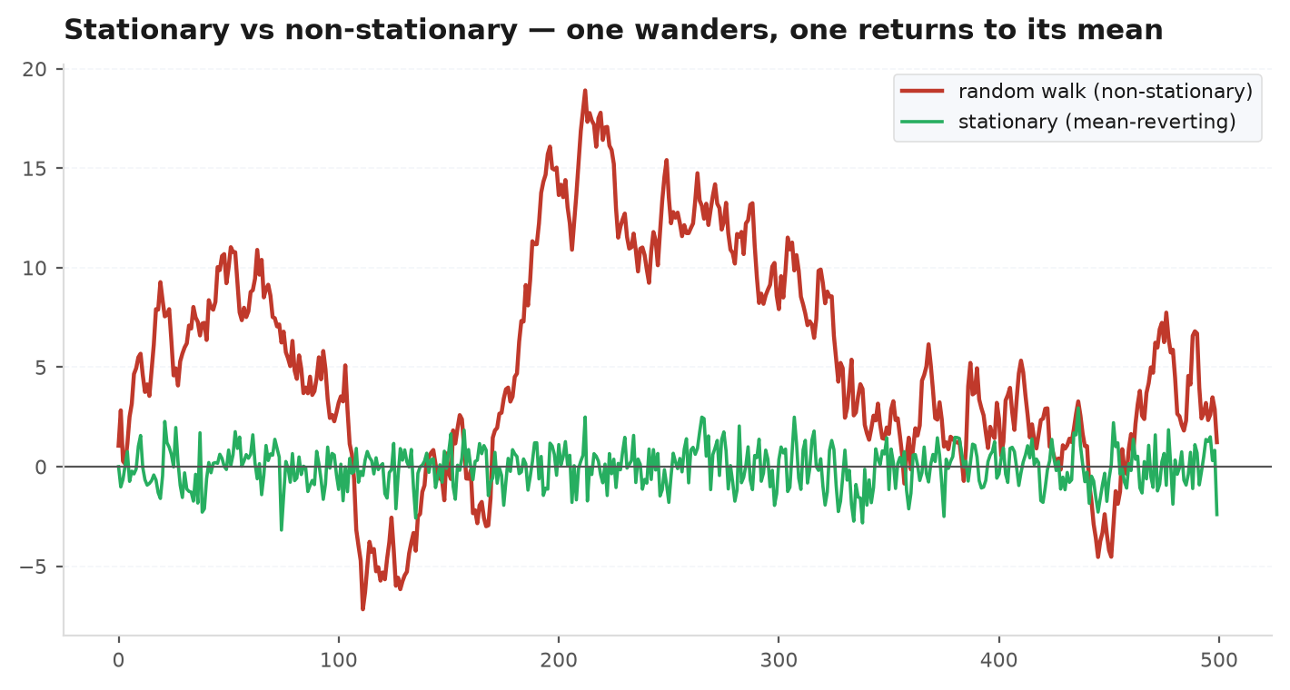

A non-stationary random-walk price path beside its stationary return series — Top: a random-walk price wanders with ever-growing variance and no fixed mean. Bottom: its log returns fluctuate around a stable zero mean — the same information, now stationary and safe to analyse.

Random walk vs mean-reversion: three tests#

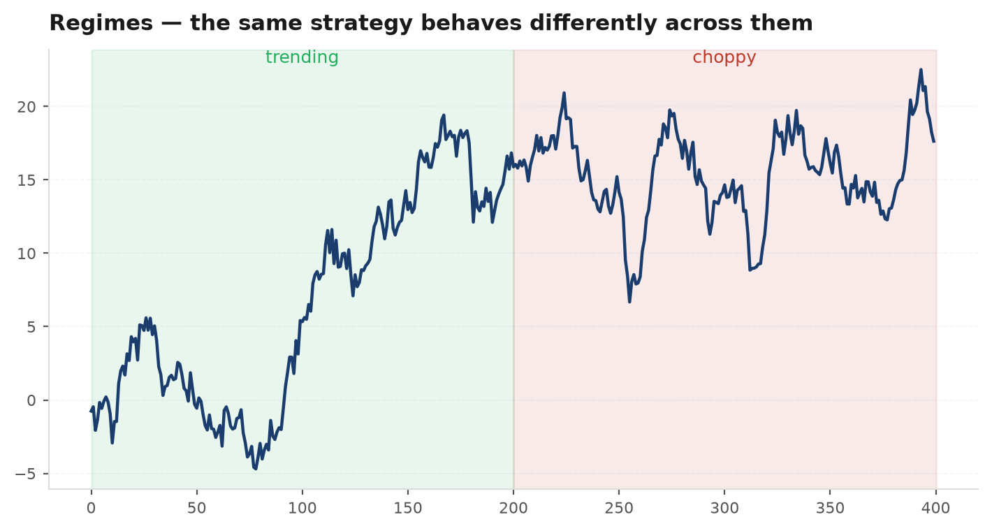
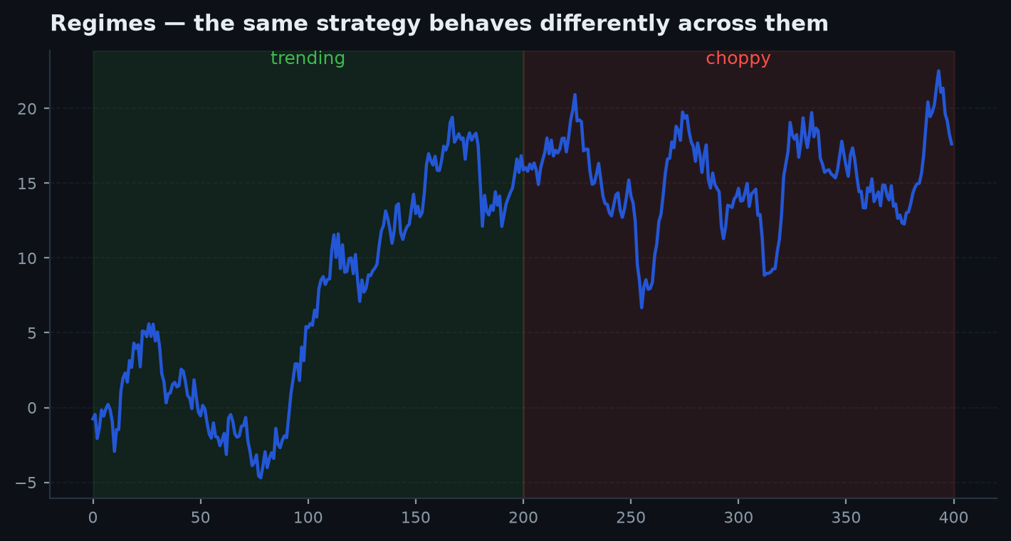
Once you can transform a series, the first question worth money is which of three worlds it lives in: a random walk (unpredictable — no edge from direction), a trending world (moves persist, so momentum pays), or a mean-reverting world (moves overshoot and snap back, so fading pays). Three complementary tests triangulate the answer.

The variance ratio#

The Lo-MacKinlay variance ratio exploits a simple fact: for a random walk, variance grows linearly with the horizon. So the variance of $k$ -period returns should be exactly $k$ times the variance of one-period returns. The ratio of the two is the statistic:

V R (k) = \frac{Var ( r _{t}^{(k)} )}{k \cdot Var ( r _{t}^{(1)} )}

Read it directly: $V R \approx 1$ is a random walk; $V R > 1$ means multi-period moves are larger than the random-walk baseline — positive autocorrelation, i.e. trend; $V R < 1$ means they are damped — negative autocorrelation, i.e. mean reversion. Sweep $k$ to see at which horizon the structure lives.

vr2 = ek.timeseries.variance_ratio(bars.close, k=2)
vr5 = ek.timeseries.variance_ratio(bars.close, k=5)
# vr > 1 -> trending on that horizon; < 1 -> mean-reverting; ~1 -> random walk

The Hurst exponent#

The Hurst exponent measures the same persistence from the scaling of dispersion across lags, boiling it into a single number in $(0, 1)$ :

$H \approx 0.5$ — a random walk (independent increments).
$H > 0.5$ — persistent / long-memory: an up move tends to be followed by another up move (trend).
$H < 0.5$ — anti-persistent: moves tend to reverse (mean reversion).

h = ek.timeseries.hurst_exponent(bars.close, max_lag=50)
# ~0.5 random walk | >0.5 persistent/trend | <0.5 mean-reverting

The ADF test#

The Augmented Dickey-Fuller test asks the sharp version of the stationarity question: does the series have a unit root(the random-walk coefficient of exactly 1)? It regresses the change on the level and tests whether the level's coefficient $γ$ is zero:

Δ x_{t} = α + γ x_{t - 1} + i = 1 \sum p δ_{i} Δ x_{t - i} + ε_{t}

The null is $γ = 0$ (a unit root — non-stationary). The test returns a t-statistic on $γ$ ; because a stationary series pulls itself back toward its mean, $γ$ is negative, and a sufficiently negative t-stat rejects the unit root. The rule of thumb: below about $- 2.86$ is significant at 5%, below $- 3.43$ at 1%. A price level typically sits near zero (fails to reject — non-stationary); its returns sit far below the threshold (stationary).

!A t-stat, not a p-value

adf_stat returns the raw t-statistic only — edgekit carries no scipy to look up an exact p-value. Compare the number to the MacKinnon critical values above. More negative = more clearly stationary.

adf_price = ek.timeseries.adf_stat(bars.close)          # near 0 -> non-stationary
adf_ret   = ek.timeseries.adf_stat(ek.timeseries.log_returns(bars.close))  # very negative -> stationary

✦Scenario: is this series mean-reverting? A two-series walk-through

You have two candidate series on the desk and want to know, before writing a single rule, which world each lives in. Series A is the BTCUSDT H4 close. Series B is a constructed spread — the residual of one index regressed on a close cousin (the stat-arb setup). You run the same three probes on each:

# Series A: BTC price level
ek.timeseries.variance_ratio(btc.close, k=5)   # -> 1.28   (>1: multi-bar moves amplify -> trend)
ek.timeseries.hurst_exponent(btc.close, 50)    # -> 0.58   (>0.5: persistent)
ek.timeseries.adf_stat(btc.close)              # -> -1.4   (near 0: unit root, can't reject random walk)

# Series B: the mean-reverting spread
ek.timeseries.variance_ratio(spread, k=5)      # -> 0.61   (<1: multi-bar moves damp -> reversion)
ek.timeseries.hurst_exponent(spread, 50)       # -> 0.34   (<0.5: anti-persistent)
ek.timeseries.adf_stat(spread)                 # -> -3.9   (well below -3.43: reject unit root, stationary)

Read together the verdict is unambiguous. Series A: VR above 1, Hurst above 0.5, ADF too shallow to reject a random walk — a trending / drifting series where a fade would get run over and a momentum idea is at least worth testing. Series B: VR below 1, Hurst below 0.5, ADF firmly past the 1% critical value — a genuinely mean-reverting spread you can build a z-score fade on. Three independent lenses agreeing is what turns a hunch into a prior. (These numbers are illustrative of the pattern, not a claim about any live instrument.)

One call for the verdict#

You rarely want to eyeball three numbers by hand. stationarity_report runs the ADF stat, the variance ratio, the Hurst exponent, and lag-1 autocorrelation together and returns a single verdict — "trending", "mean-reverting", or "random-walk" — plus the raw components so you can see why.

rep = ek.timeseries.stationarity_report(bars.close)
# {"adf_stat": ..., "variance_ratio": ..., "hurst": ...,
#  "autocorr_lag1": ..., "verdict": "trending" | "mean-reverting" | "random-walk"}
if rep["verdict"] == "random-walk":
    print("no directional edge here — don't fit a trend or reversion rule")

→A verdict is a prior, not a strategy

A “trending” verdict says a momentum idea is worth testing, not that it works — the series can still fail the full validation gauntlet on costs or out-of-sample. Treat the report as a filter on where to spend your research time, then prove the edge properly in Part IV.

Autocorrelation: the memory of a series#

The variance ratio and Hurst exponent both summarise autocorrelation — the correlation of a series with a lagged copy of itself. The ACF and PACF show it lag by lag, which is how you read the actual memory structure rather than a single scalar.

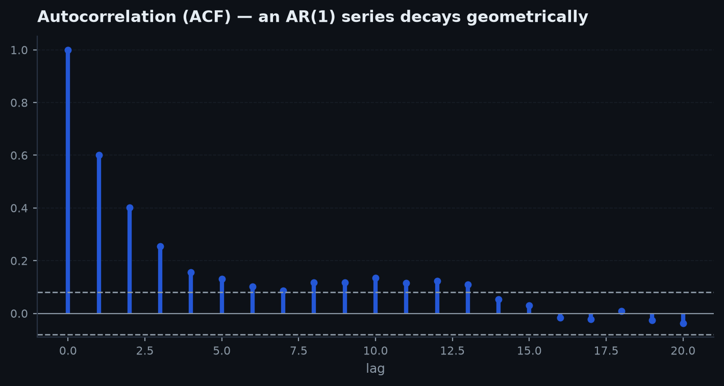
The autocorrelation function (ACF) at lag $k$ is the correlation between $r_{t}$ and $r_{t - k}$ . By construction $ACF (0) = 1$ . A slow, gradual decay signals persistence; a sharp cut-off after a few lags signals short-memory (moving-average) structure; bars that are all inside the noise band signal white noise — no linear predictability.

ρ_{k} = \frac{\sum _{t} ( r _{t} - r ˉ ) ( r _{t - k} - r ˉ )}{\sum _{t} ( r _{t} - r ˉ ) ^{2}}

The partial autocorrelation function (PACF) gives the correlation at lag $k$ after removing the influence of all shorter lags. The division of labour is the classic Box-Jenkins reading: the PACF cutting off after lag $p$ suggests an AR(p) process, while the ACF cutting off after lag $q$ suggests an MA(q).

Significance is judged against the white-noise band. Under the null of no autocorrelation, each coefficient is approximately normal with standard error $1/ n$ , so the two-sided 95% band is:

\pm \frac{1.96}{n}

Bars poking outside that band are the ones worth a second look; bars inside it are noise. edgekit computes both functions directly (the PACF via Durbin-Levinson recursion — no statsmodels):

ac = ek.timeseries.acf(rets, nlags=40)     # ac[0] == 1
pc = ek.timeseries.pacf(rets, nlags=40)    # partial autocorrelations
band = 1.96 / len(rets) ** 0.5             # the +/- significance band

lag1 = ek.timeseries.autocorr(rets, lag=1) # single-lag convenience form

And to ask “is there anyautocorrelation across the first several lags at all?” in one shot, the Ljung-Box portmanteau test pools them:

lb = ek.timeseries.ljung_box(rets, lags=10)
# lb == {"stat": Q, "dof": 10}; compare Q to a chi-squared(dof) — a large Q rejects white noise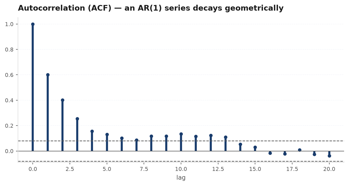

ACF and PACF of a return series with the significance band — ACF (top) and PACF (bottom) with the +/-1.96/sqrt(n) band shaded. Bars inside the band are indistinguishable from white noise; a spike outside it at a given lag is where predictable structure lives.

Volatility clustering: returns are not iid#

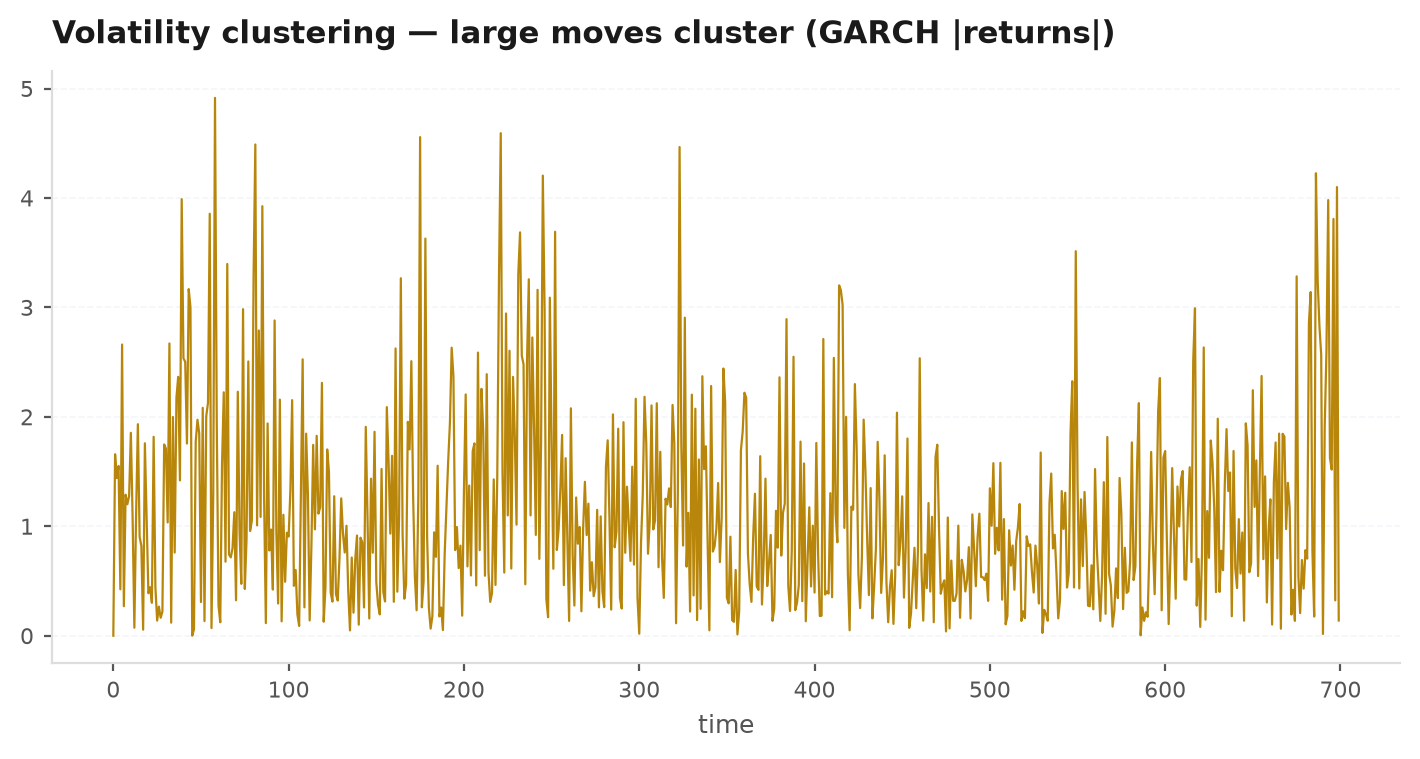
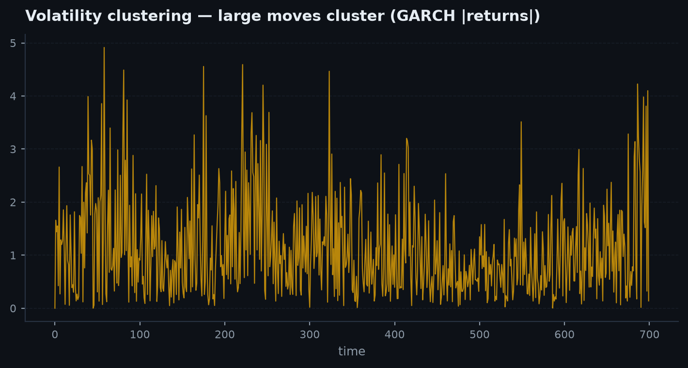
Here is the twist that shapes almost every real strategy. Run the ACF on returns and you usually find very little — direction is close to unpredictable. Run it on squared (or absolute) returns and you find strong, slowly-decaying autocorrelation. That is volatility clustering: large moves cluster with large moves and calm with calm, even when the signof the next move is unpredictable. The famous one-liner is that returns are “serially uncorrelated but not independent.”

This is the empirical fact GARCH-family models formalise — tomorrow's variance is a weighted blend of a long-run level, yesterday's variance, and yesterday's squared shock — and it is why a single fixed stop distance is fragile: the size of a “normal” move is itself time-varying. edgekit gives you the practical estimators without the full GARCH fit. The RiskMetrics EWMA recursion is the workhorse:

σ_{t}^{2} = λ σ_{t - 1}^{2} + (1 - λ) r_{t}^{2}, λ = 0.94

Because recent squared returns carry more weight, EWMA vol turns on a dime when a shock hits — much faster than a flat rolling window, which dilutes the shock across the whole lookback. Use it to size risk in volatility units so a stop widens in stress and tightens in calm.

ewma = ek.timeseries.ewma_volatility(rets, lam=0.94)     # RiskMetrics, fast-reacting
roll = ek.timeseries.rolling_volatility(rets, 20, periods_per_year=252)  # annualised
rv   = ek.timeseries.realized_vol(rets, window=20)       # vol actually delivered

# confirm the clustering: autocorrelation of SQUARED returns is strongly positive
lb_sq = ek.timeseries.ljung_box(rets ** 2, lags=10)

Scenario (why a fixed stop breaks). On BTCUSDT you run ljung_box(rets, 10) and get Q ≈ 9 against a chi-squared(10) — inside the noise band, direction is unpredictable. Then you run it on rets ** 2 and get Q ≈ 140 — a screaming rejection of white noise. Same series, opposite verdicts: the sign of tomorrow's move is a coin flip, but its sizeis highly forecastable. That is why the EWMA vol you'd have sized a stop off in the calm June regime (say 0.9% daily) is useless the day a 3% shock lands — the estimate reprices within a bar or two, and a stop pinned to the old number gets swept.

Return series showing bursts of high and low volatility with an EWMA volatility overlay — Volatility clusters: quiet stretches and violent stretches group together. The EWMA estimate (overlay) tracks the regime, spiking as a shock arrives and decaying through the calm that follows.

Seasonality & decomposition#

Some series carry a repeating calendar rhythm — a day-of-week pattern in equity-index returns, an hour-of-session pattern in intraday volume. seasonal_decompose splits a series into three additive parts over a fixed period so you can see the cycle on its own:

x_{t} = trend_{t} + seasonal_{t} + resid_{t}

The trend is the slow drift, the seasonal component is the repeating cycle of length period, and the residual is what neither explains. If the seasonal component is small relative to the residual, there is no reliable cycle to trade — the honest and common outcome.

dec = ek.timeseries.seasonal_decompose(daily_ret, period=5)   # weekly cycle on daily bars
# dec == {"trend": Series, "seasonal": Series, "resid": Series}
dec["seasonal"]   # the repeating component; compare its scale to dec["resid"]

Scenario (a “Monday effect” that isn't). You decompose daily US500 returns with period=5and the seasonal component shows Monday averaging −0.06% and Wednesday +0.05%. Tempting. But the residual's daily standard deviation is 1.1% — the seasonal swing is one-twentieth the noise it swims in. At the desk that means the “pattern” would be buried by a single ordinary day's move: not a tradeable cycle, just the sample's particular wobble. A seasonal component only earns a second look when its amplitude is a meaningful fraction of the residual, which is the honest-and-usually-disappointing outcome here.

A series decomposed into trend, seasonal, and residual components — An additive decomposition: the slow trend, the repeating seasonal cycle, and the residual noise. A seasonal component that is dwarfed by the residual is not a tradeable pattern.

✕Analysis describes the past — it does not forecast the future

Every statistic here is estimated on a finite historical sample. A verdict, an ACF spike, a seasonal bump can all be artefacts of the particular window you looked at. The tools tell you where structure might be; whether it survives is decided out-of-sample, under costs, in the validation gauntlet. Never size a position off a diagnostic alone.

Where this leads#

You now have the vocabulary to describe a series honestly: stationary or not, trending or reverting or random, which lags carry memory, whether volatility clusters, whether a calendar cycle exists. The next step is turning that description into inputs a strategy can act on — without smuggling the future into the past.

Next: Feature engineering — how make_features turns raw OHLC into a causal feature matrix, and the leakage traps that quietly destroy otherwise-sound models.