Event studies & seasonality

Does the market rally after big down days? Do earnings surprises drift? Is there really a Monday effect? Each is a claim that returns behave differently around a defined event — and the event study is the classical design for testing it: align every occurrence on a common clock, average out the noise, and ask whether what remains is distinguishable from zero. It is a beautiful machine, and — because you can define infinitely many events — one of the easiest to fool yourself with.

✦Intuition — stacking the days on top of each other

Any single post-event window is dominated by noise: the market fell 2% on Tuesday and rose Wednesday — so what? The event study’s move is to collect every 2%-down day in the sample, cut out the window of days around each one, stack the windows on a shared axis (day 0 = the event), and average across the stack. Idiosyncratic noise cancels at rate $N$ ; any systematic reaction survives the averaging. The design turns one unanswerable anecdote into $N$ repeated experiments. Everything else in this chapter — abnormal returns, CAR, its variance, the bootstrap null — is bookkeeping to make the averaging honest.

The design: estimation window vs event window#

For each event at date $τ$ , define two disjoint windows on the event clock:

Estimation window — for example the 60 days ending beforethe window of interest, used only to estimate what “normal” looks like: the benchmark mean return $μ^$ and variance $σ^^{2}$ .
Event window — relative days $t \in [t_{1}, t_{2}]$ around the event (say $- 5$ to $+ 10$ ), where the hypothesised reaction lives. It must never overlap the estimation window, or the event contaminates its own benchmark.

The abnormal return is the raw return minus the benchmark. The simplest benchmark is the estimation-window mean (mean-adjustment, $A R_{i, t} = r_{i, t} - μ^_{i}$ ); the next step up is market-adjustment, subtracting $α^_{i} + β^_{i} r_{m, t}$ from a CAPM fit on the estimation window, so a market-wide move on the event day is not mistaken for a reaction. Either way the logic is identical: normal behaviour is estimated out of the event window and subtracted in it.

Defining the event without peeking#

The event definition itself must be causal: computable at the moment it fires, from information available then. “Daily return below $- 2%$ ” qualifies. “Days in the worst 5% of the sample” does not — the threshold uses the whole sample, so early events are defined by data from their own future, the same look-ahead leak that poisons backtests. A clean mechanical option is the CUSUM filter, ek.timeseries.cusum_breaks: it accumulates standardised surprises and fires an event when the running sum crosses a threshold, using only past data — and it naturally spaces events out, which limits the window-overlap problem below.

AAR and CAR#

Average the abnormal returns across the $N$ events at each relative day, then accumulate through the window:

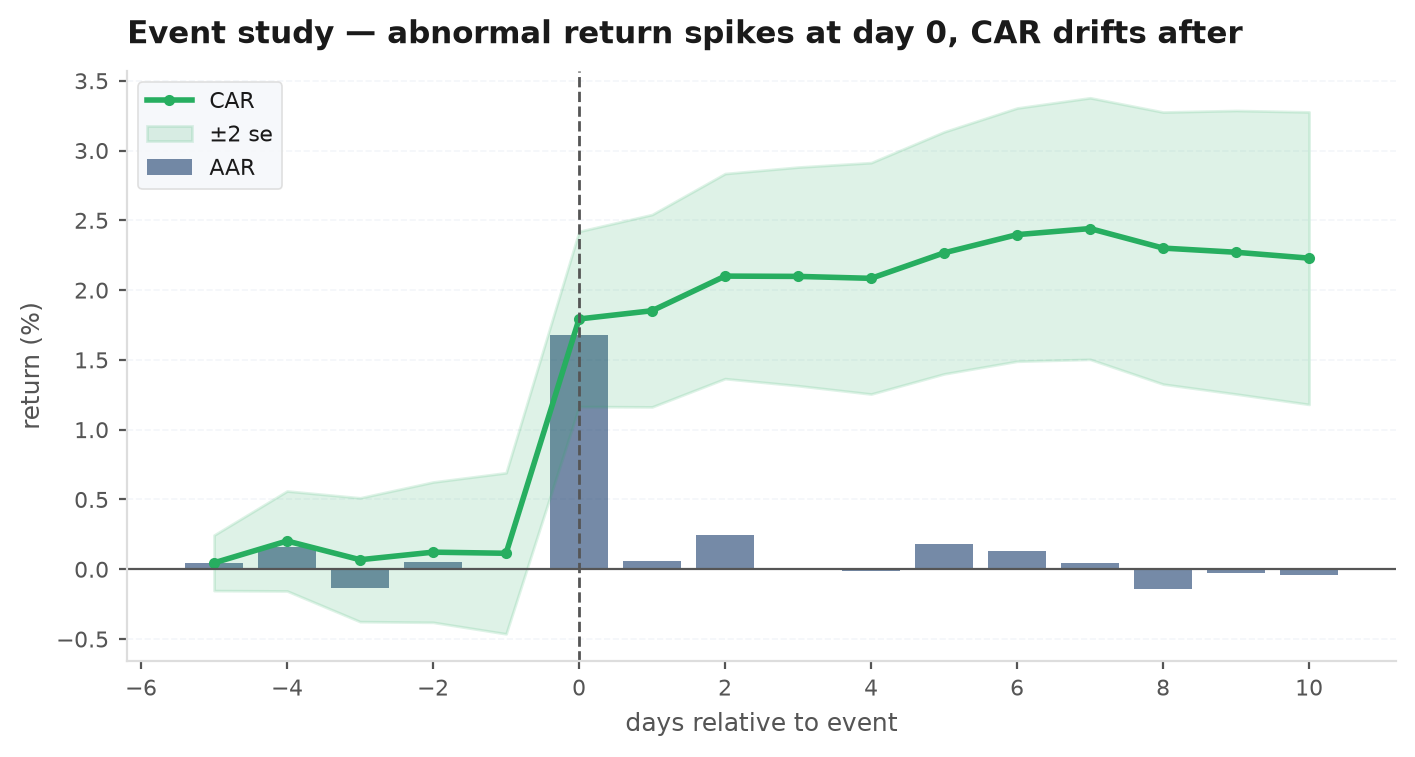
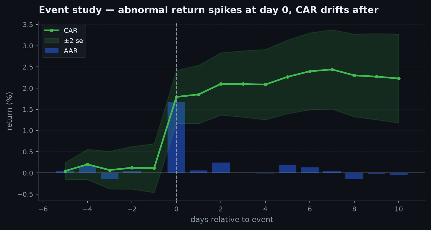
AA R_{t} = \frac{1}{N} i = 1 \sum N A R_{i, t}, C A R_{(t_{1}, t_{2})} = t = t_{1} \sum t_{2} AA R_{t} .

The average abnormal return (AAR) shows the shape of the reaction day by day; the cumulative abnormal return (CAR) is the total drift over the window — the number a trading rule could actually have captured. A real effect shows up as a CAR path that departs from zero after day 0 and stays departed; a CAR that wanders back is noise doing what noise does.

→CAR is a backtest in miniature

A rule that buys at the close of day

t_{1} - 1

after each event and exits at day

t_{2}

earns, on average, exactly

C A R_{(t_{1}, t_{2})}

per event — before costs. That translation is worth doing early: a “highly significant” 15bp CAR on events that fire monthly is under 2% a year of gross edge, gone after one spread crossing. Statistical and economic significance are separate hurdles, and an event effect must clear both.

✦Derivation — the variance of CAR, and the t-test on it

Under the null there is no event effect: each $A R_{i, t}$ is just noise with variance $σ^{2}$ (estimated from the estimation window). If events are independent of each other, averaging across $N$ events divides the variance by $N$ :

Var (AA R_{t}) = \frac{σ ^{2}}{N} .

If daily abnormal returns are also serially uncorrelated within the window, the variance of a sum is the sum of variances, so over a window of $L = t_{2} - t_{1} + 1$ days:

Var (C A R_{(t_{1}, t_{2})}) = t = t_{1} \sum t_{2} Var (AA R_{t}) = \frac{L σ ^{2}}{N},

t_{C A R} = \frac{C A R _{(t_{1}, t_{2})}}{L σ ^{2} / N} .

Read the denominator. Detectability improves with $N$ (more events) but degrades with $L$ (longer windows accumulate noise as fast as they accumulate effect). A 30bp drift over 3 days is far easier to detect than the same 30bp smeared over 30 days. And both independence assumptions are load-bearing: overlapping event windows (clustered events) correlate the $A R_{i, t}$ across $i$ and shrink the effective $N$ — the same effective-sample-size trap as in cross-sectional inference.

Average cumulative abnormal return plotted against event-relative day, flat before day zero then drifting upward after the event with a confidence band — The event study in one picture. Day 0 is the event; the line is the cumulative abnormal return averaged over all events; the band is ± 2 standard errors from the CAR variance formula. A real effect departs from zero at day 0 and holds outside the band — a line that wobbles inside the band is the null doing its work.

The bootstrap null band#

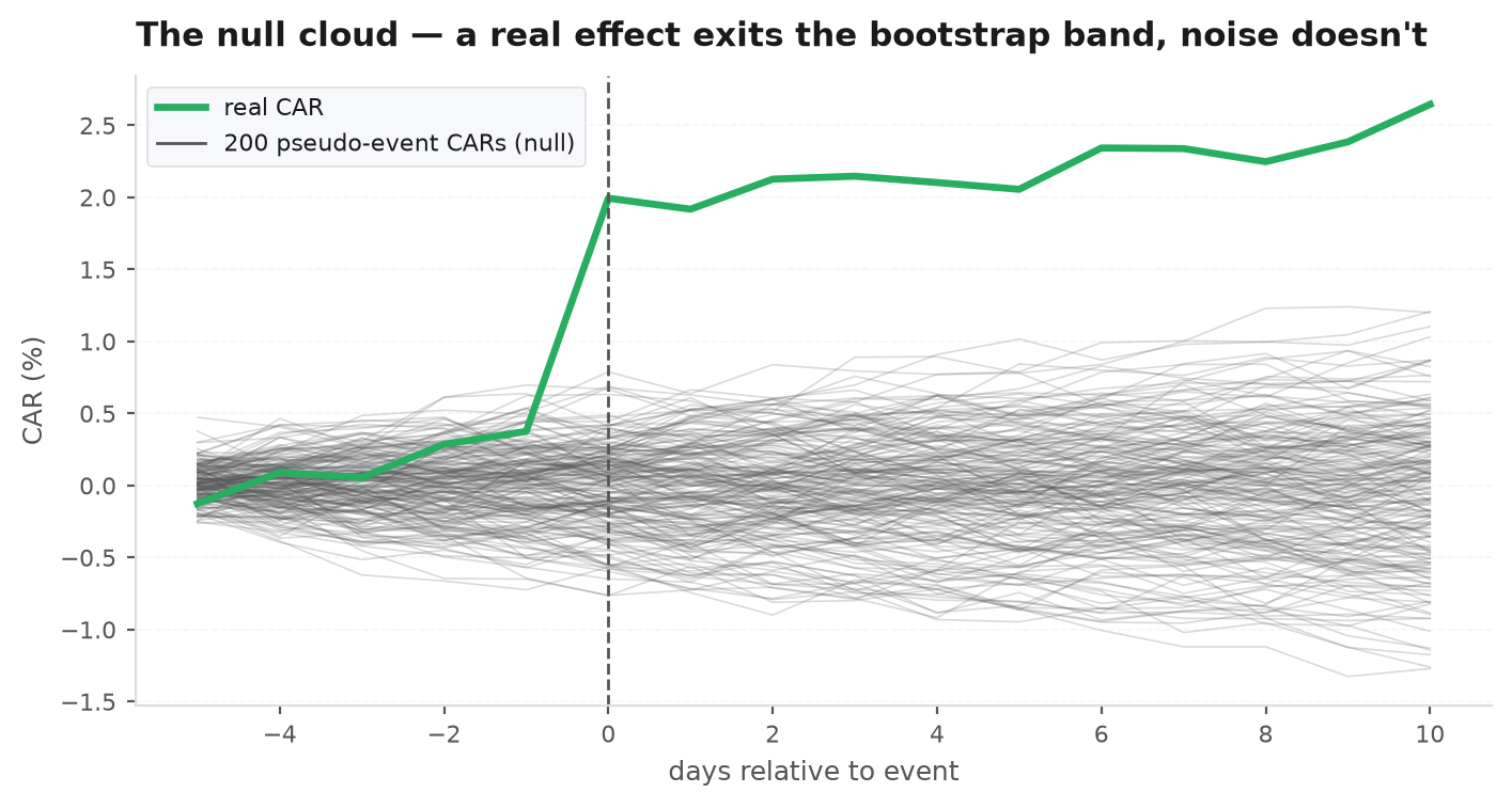
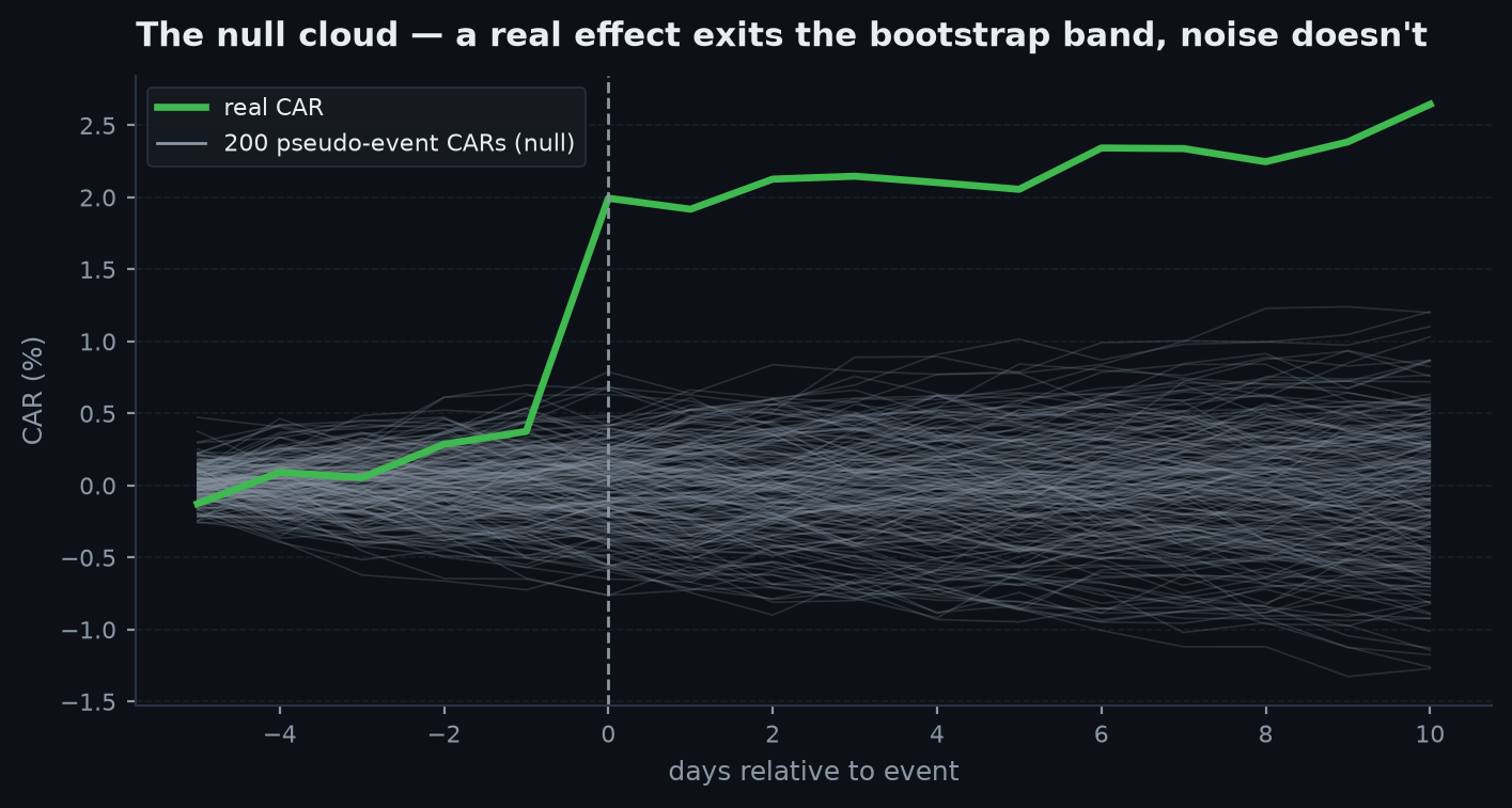
The analytic t-test leans on Gaussian, independent noise — both dubious for daily returns. The nonparametric alternative asks the question directly: what CAR paths do randomly chosen non-event dates produce? Draw $N$ fake event dates at random, compute the CAR exactly as for the real events, repeat a few thousand times, and read the 2.5% and 97.5% quantiles at each relative day. That is a null bandbuilt from the actual return distribution — fat tails, clustering and all. A real CAR that exits the band is significant on the data’s own terms; this is the same placebo logic as the permutation tests in the gauntlet.

The observed CAR path compared against a funnel of bootstrap CAR paths from random placebo event dates, with the observed path escaping the funnel — Bootstrap null band. Grey paths are CARs computed on randomly drawn placebo event dates — what 'no effect' genuinely looks like on this data, with its real fat tails and clustering. The observed CAR (dark line) is only interesting where it escapes the funnel. Note how wide the funnel is: daily noise makes impressive-looking drifts routinely by chance.

event_study.py

import edgekit as ek

# 1. define events mechanically — here, CUSUM breaks on the return series
events = ek.timeseries.cusum_breaks(close_returns, threshold=5.0)

# 2. run the study: market-adjusted ARs, AAR/CAR, analytic t-stat
es = ek.factors.event_study(returns, events,
                            window=(-5, 10), estimation=60)
es["aar"]        # Series indexed by relative day
es["car"]        # cumulative abnormal return path
es["t_car"]      # t-stat on the full-window CAR
es["n_events"]   # how many events actually had clean windows

# 3. bootstrap the null: same study on random placebo dates
rng = ek.core.bootstrap_rng(seed=11)
null_cars = []
for _ in range(2000):
    fake = list(rng.choice(len(returns) - 20, size=es["n_events"]))
    null_cars.append(ek.factors.event_study(
        returns, fake, window=(-5, 10), estimation=60)["car"])

✦Scenario — does the market rally after 2%-down days?

Define the event as “daily return below $- 2%$ ” and suppose a 10-year daily sample contains $N = 48$ such days. To see what a detectable effect looks like, inject one: add a $+ 30$ bp drift spread over the 3 days after each event in a simulated series with daily $σ = 1%$ . The study should recover $C A R_{(1, 3)} \approx 0.30%$ , and the t-stat follows from the variance formula:

t_{C A R} = \frac{0.0030}{3 \times ( 0.01 ) ^{2} /48} = \frac{0.0030}{0.00250} \approx 1.2.

A genuinely injected 30bp bounce and the design cannot see it with 48 events — the noise floor $L σ^{2} / N = 25$ bp is nearly the size of the effect. You would need roughly $N \approx 130$ events (or a tighter window) before $t > 2$ . Now run it in reverse: on real data, a reported $C A R = 0.5%$ after down days, with $t = 2.0$ , is exactly the size of finding the bootstrap band routinely produces — and 2%-down days cluster in crashes, so the windows overlap and the effective $N$ is well below 48. The honest summary: with rare events, daily noise, and clustering, most tradable-sized effects are statistically invisible — and most “statistically visible” ones are artifacts.

Seasonality is a repeated event study#

Every calendar effect — Monday effect, turn-of-month, December rally, options-expiry week — is an event study where the “event” is a date pattern rather than a market condition. The same machinery applies verbatim: the events are all Mondays, the window is the day itself, AAR is the average Monday return, and the null band comes from bootstrapping random weekdays. What changes is the multiplicity: the calendar offers an enormous menu of patterns to test, which is precisely the problem.

→The Monday effect, run through the machinery

Ten years of daily data holds about $N \approx 500$ Mondays. Suppose Mondays averaged $- 3$ bp against $+ 5$ bp for other weekdays — an 8bp gap, the classic finding. With daily $σ = 1%$ , the standard error of the Monday mean is $σ / N = 1%/ 500 \approx 4.5$ bp, so the gap prints $t \approx 1.3$ — unremarkable. The original studies reached significance with much longer samples; on post-publication data the effect flipped sign. Five hundred repetitions of a tiny effect against 1% daily noise is still a weak experiment — seasonality claims need either decades of data or effect sizes that would be visible to the naked eye.

The honesty section: infinite events, one dataset#

The event-study design has a silent free parameter: the definition of the event. Down 2% or down 3%? Close-to-close or intraday? Rally over 1 day, 3 days, or 10? Each choice is a new hypothesis, and the combinatorics explode:

Menu	Choices	Cumulative tests
Event threshold	-1%, -2%, -3%, -5%	4
Response window	(0,1), (1,3), (1,5), (1,10)	16
Adjustment	mean, market, none	48
Calendar variants	Mondays, month-end, expiry, pre-holiday…	300+

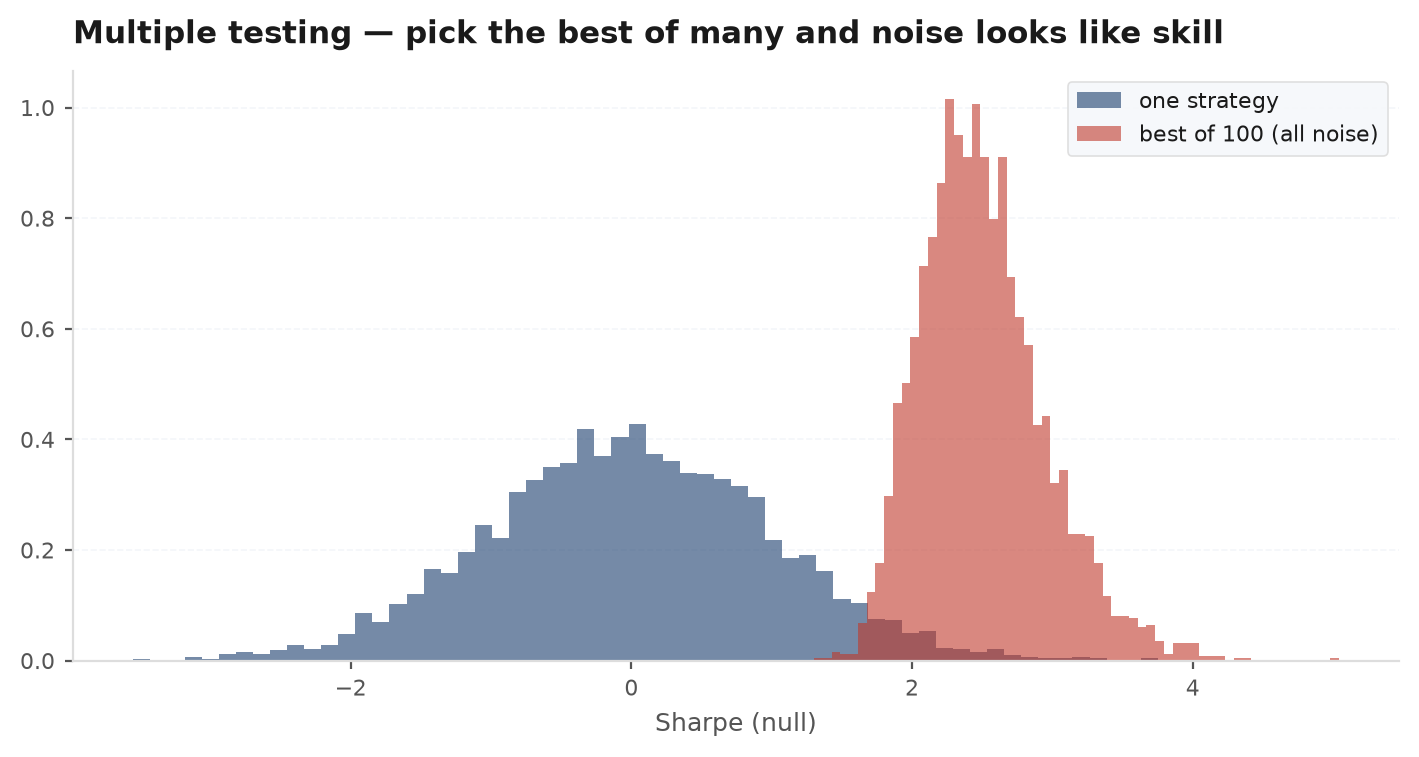
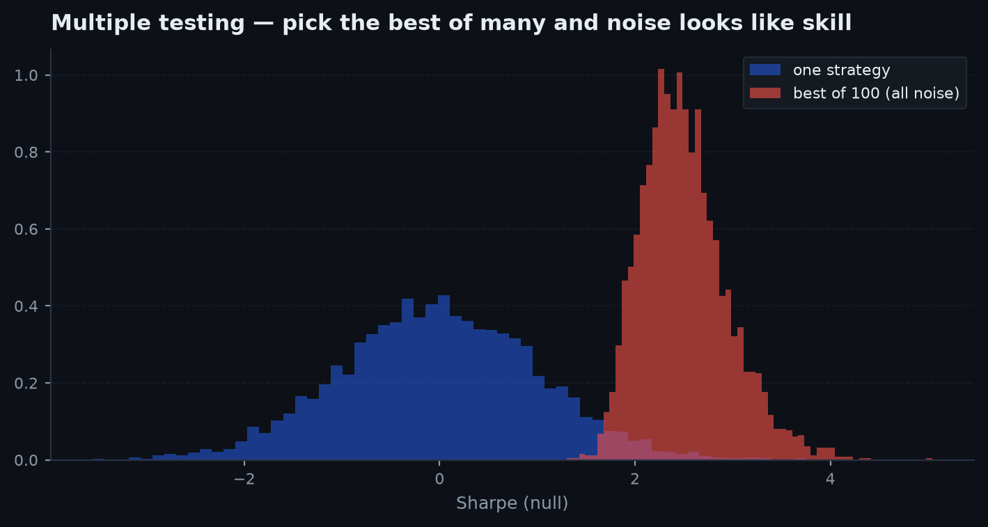
At 300 implicit tests, the 5% false-positive rate guarantees a shelf of “significant” effects in pure noise — the same arithmetic as the multiple-testing chapter, now wearing a calendar. This is how the finance literature accumulated dozens of seasonal anomalies that evaporated on fresh data.

The probability of at least one false positive rising rapidly with the number of hypotheses tested at the 5% level — The multiple-testing curve, revisited for calendars. Each event definition, window, and adjustment is one more draw at the 5% false-positive slot machine; by a few dozen implicit tests, finding 'significant' seasonality in pure noise is close to guaranteed. The bar must rise with the size of the menu you searched.

!Pre-register the event, then look

The defence is procedural, not statistical: write down the event definition, window, and adjustment beforetouching the data — a pre-registration mindset. One hypothesis, stated in advance, tested once, with the bootstrap band as the referee. If instead you searched the menu, say so and deflate accordingly (Bonferroni across the menu size is the crude-but-honest correction). An effect that only appears for “down 2.5% days, 4-day response, mean-adjusted” is not a discovery; it is a coordinate in search space. Put every survivor through why backtests lie and the gauntlet before it touches capital.

Next: from reactions around events to a return source that needs no event at all — the yield an asset pays you just for holding it. Carry & term structure.