The volatility surface

In volatility trading you inverted one option price into one implied vol. But an option market quotes hundreds of prices at once — every strike, every expiry — and inverting them all yields a surface: implied volatility as a function of moneyness and time. This chapter maps that surface — why it smiles, the no-arbitrage constraints that discipline its shape, the SVI parameterisation that fits it, the variance swap that trades a whole slice of it — and closes with the fundamental theorem of vol trading: the delta-hedging P&L identity that turns the surface into a market for realized-vs-implied bets.

✦Intuition — the surface is a table of prices for insurance

Each point on the surface answers one question: what does the market charge, per unit of volatility, to insure a move to this price level by this date? Reading across strikes tells you which outcomes the market fears (downside protection costs more — the skew); reading across expiries tells you when it fears them (event dates bulge; long-dated vol reverts to a long-run mean). A single Black-Scholes $σ$ flattens this rich object to one number. The surface is the market’s entire probability distribution for the underlying, encoded in vol units — and a vol trader’s job is to find the coordinates where that encoding disagrees with reality.

From one vol to a surface#

Fix an expiry and sweep across strikes: implied vol traces the smile (in equities, a downward skew — OTM puts dearest). Fix a strike and sweep across expiries: vol traces a term structure, typically upward-sloping in calm markets (long-dated uncertainty accumulates) and inverted in panics (the crash is priced as imminent, not chronic). Put the two together and you have $σ_{imp} (K, T)$ , the surface.

Implied volatility versus strike forming a downward-tilted smile, steeper on the put side — One expiry slice of the surface: the smile. Black-Scholes predicts a flat line; the market prints a skewed U. The two standard explanations — fat-tailed returns and the leverage effect — both raise the price of downside strikes relative to the Gaussian benchmark.

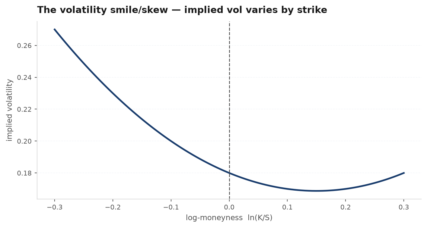
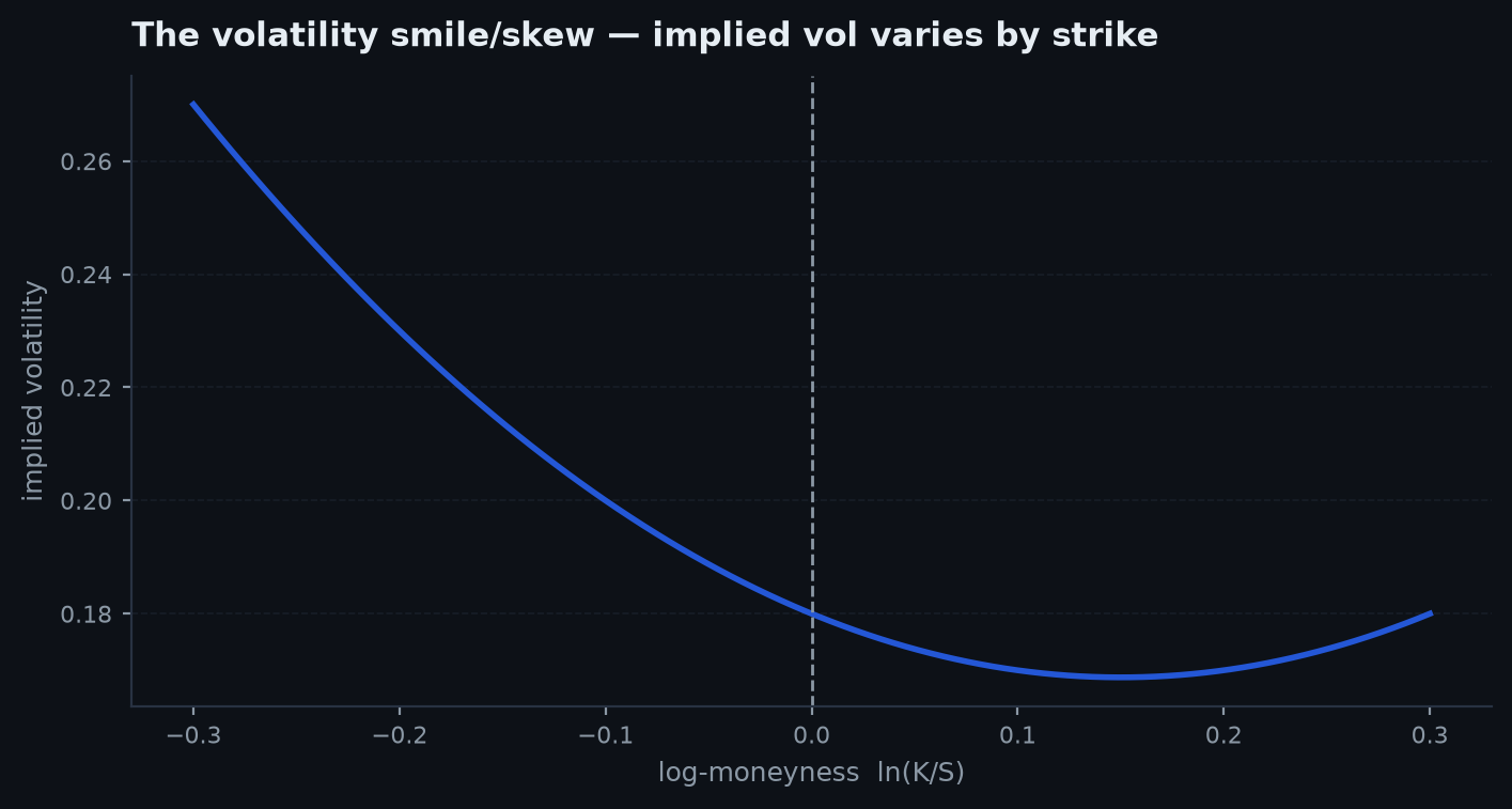
Why does the smile exist at all? Two mechanisms, both departures from geometric Brownian motion:

Fat tails. Real returns jump. Far-OTM options are bets on the tails, and heavy tails make them worth more than any single lognormal density allows — so inverting their prices through Black-Scholes forces the wing vols up. The jumps chapter makes this quantitative: Merton jump-diffusion prices, pushed back through the BS formula, produce a smile mechanically.
The leverage effect. Volatility rises when prices fall (negative spot-vol correlation), so down-moves arrive with extra variance. Puts pay off precisely in the high-vol state, making them worth more — the asymmetry of the smile, the skew.

The natural coordinates are log-moneyness $k = ln (K / F)$ (strike over forward — comparable across spot levels and expiries) and total implied variance:

w (k, T) = σ_{imp}^{2} (k, T) T .

Total variance is the quantity no-arbitrage speaks about. Two constraints, stated intuitively: butterfly — at fixed $T$ , the smile cannot be so convex or so steep that the implied probability density goes negative (a butterfly spread of calls has a non-negative payoff, so it must have a non-negative price); and calendar — total variance must be non-decreasing in $T$ at fixed moneyness (a longer option spans every outcome the shorter one does; if $w$ ever fell with maturity you could buy the long, sell the short, and lock in a riskless profit). A fitted surface violating either is not a market view — it is an error.

Raw SVI: five parameters per expiry#

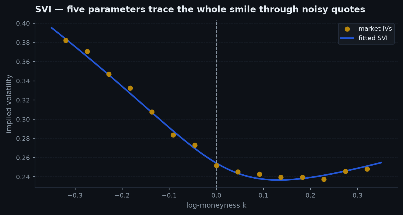
You cannot trade a scatter of noisy quotes; you need a smooth curve with few parameters. The industry standard is Gatheral’s raw SVI(“stochastic volatility inspired”) form for total variance at one expiry:

w (k) = a + b (ρ (k - m) + (k - m)^{2} + σ^{2}) .

Each parameter moves one feature of the smile:

Parameter	Controls	Effect when increased
a	Overall level	Lifts the whole smile (total variance floor)
b	Wing slope	Steepens both wings — more smile
ρ ∈ (−1, 1)	Asymmetry	ρ < 0 tilts the smile down to the right: equity skew
m	Horizontal shift	Slides the vertex along log-moneyness
σ > 0	Vertex curvature	Rounds the bottom — smaller σ, sharper kink at the money

The wings grow linearly in $∣ k ∣$ (slopes $b (1 \pm ρ)$ ), which matches both observation and the theoretical bound that total variance can grow at most linearly in log-moneyness. edgekit fits the five parameters with a built-in Nelder–Mead search — no gradients, pure numpy.

svi.py

import numpy as np
import edgekit as ek

# market quotes for one expiry: strikes -> implied vols
k = np.log(strikes / fwd)                  # log-moneyness
params = ek.options.svi_fit(k, ivs, t=0.25)
params                                     # {"a","b","rho","m","sig"}

# evaluate the fitted smile on a dense grid
grid = np.linspace(-0.4, 0.4, 101)
smile = ek.options.svi_iv(params, grid, t=0.25)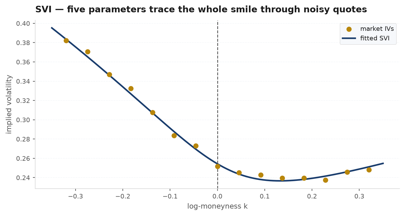

Market implied vol quotes as scattered points with the fitted five-parameter raw SVI curve passing smoothly through them — Raw SVI fitted to one expiry's quotes. Five parameters reproduce the level (a), wing steepness (b), skew (rho), vertex location (m) and curvature (sig) of the whole smile. The fit smooths quote noise and lets you interpolate a consistent vol at any strike — but always check the fitted slice against the butterfly and calendar constraints.

Variance swaps: trading a whole slice#

A variance swap pays realized variance minus a fixed strike $K_{var}$ at expiry — the purest realized-vs-implied instrument, no deltas, no strikes, no rebalancing. Its fair strike is readable directly off the smile.

✦Derivation sketch — the fair strike from the strip of options

By Itô, the gap between realized variance and the log-contract payoff integrates cleanly: for any continuous path,

\int_{0}^{T} σ_{t}^{2} d t = 2 \int_{0}^{T} \frac{d S _{t}}{S _{t}} - 2 ln \frac{S _{T}}{S _{0}} .

The first term is a self-financing futures strategy (worth zero risk-premium in expectation); everything reduces to pricing the log contract $- ln (S_{T} / F)$ . Any smooth payoff can be replicated statically by a portfolio of calls and puts across strikes, and for the log payoff the required weight at strike $K$ is $1/ K^{2}$ — OTM puts below the forward, OTM calls above it. Hence

K_{var} = \frac{2 e ^{r T}}{T} [\int_{0}^{F} \frac{P ( K )}{K ^{2}} d K + \int_{F}^{\infty} \frac{C ( K )}{K ^{2}} d K] .

Two readings. First, the fair variance strike is an average over the entire smile — the wings enter with weight $1/ K^{2}$ , so a variance swap is implicitly long the skew, and $K_{var}$ sits above ATM implied vol whenever the smile is not flat. Second, this is exactly the VIX construction: the VIX is the square root of the 30-day $K_{var}$ computed from the S&P strip. edgekit’s variance_swap_strike discretises the integral over your strike grid.

varswap.py

import edgekit as ek

kvar = ek.options.variance_swap_strike(strikes, ivs, s=100.0,
                                       t=30/365, r=0.04)
fair_vol = kvar ** 0.5      # in vol units — the 'VIX' of this strip
# short the swap: receive kvar, pay realized variance at expiry

The fundamental theorem of vol trading#

Most vol trades are still expressed with plain options, delta-hedged. What exactly does the hedger earn? The answer is the single most important identity in this part of the book.

✦Derivation — hedging P&L = ½ Γ S² (σ²_real − σ²_imp) dt

Sell an option at implied vol $σ_{imp}$ , and delta-hedge using the Black-Scholes delta computed at that same vol. Over a step $d t$ the hedged book (short option, long $Δ$ stock) changes by the Taylor expansion terms delta does not cancel:

d Π = - Θ d t - \frac{1}{2} Γ (d S)^{2} + O (d t^{3/2}) .

But the option was priced at $σ_{imp}$ , and the Black-Scholes equation ties its theta to its gamma at that vol (ignoring rates for clarity):

Θ = - \frac{1}{2} Γ S^{2} σ_{imp}^{2} .

Meanwhile the world moves at realized vol: $(d S)^{2} = σ_{real}^{2} S^{2} d t$ . Substitute both:

d Π = \frac{1}{2} Γ S^{2} (σ_{imp}^{2} - σ_{real}^{2}) d t,

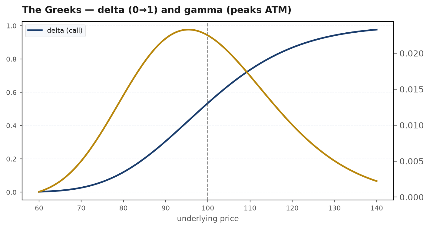
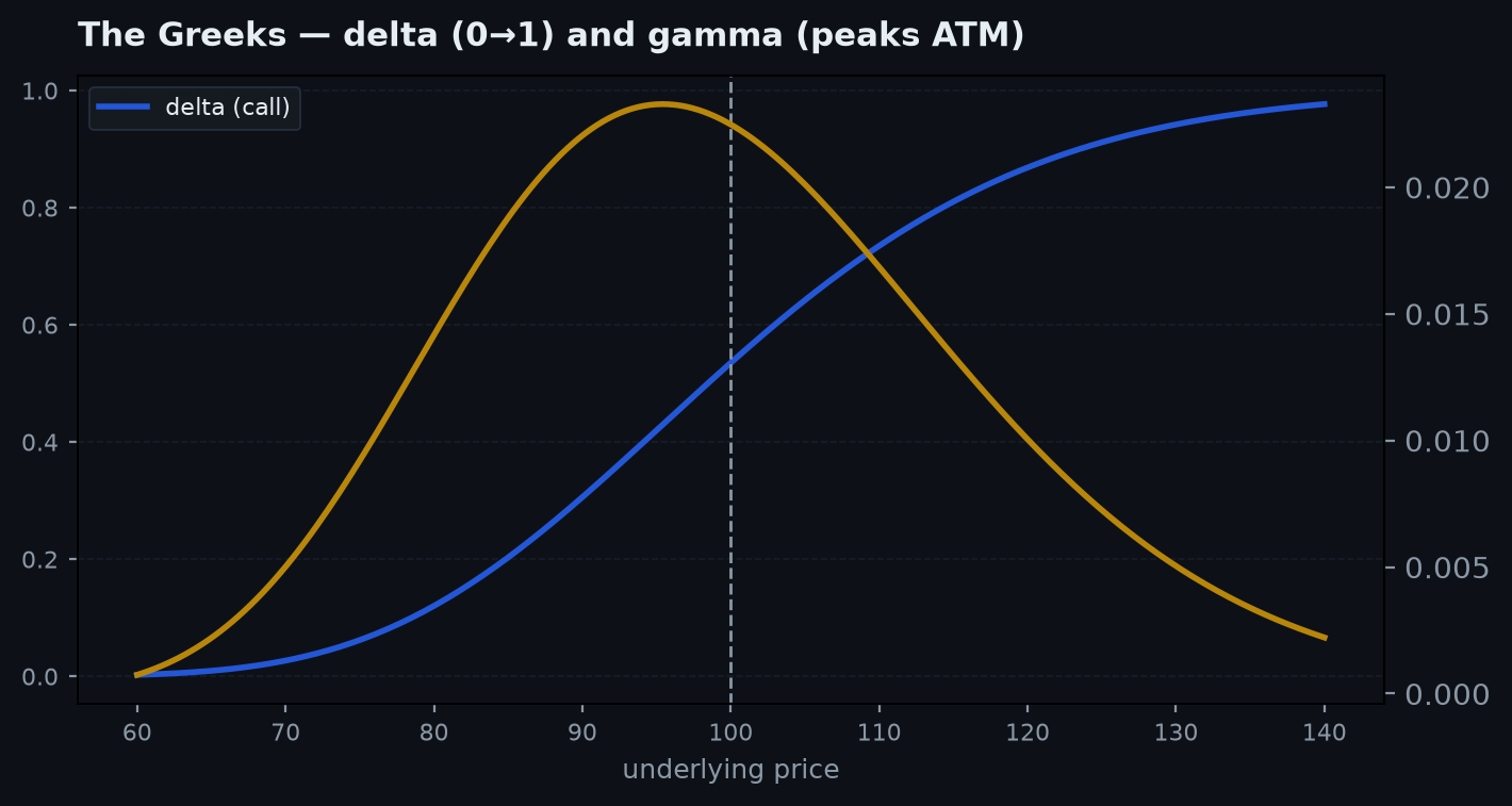
and the buyer’s side is the negative: a hedged long option earns $\frac{1}{2} Γ S^{2} (σ_{real}^{2} - σ_{imp}^{2}) d t$ each step. Every Greek except the vol gap has vanished. Direction is hedged away; what remains is gamma-weighted variance mispricing, accrued continuously. This is why implied-vs-realized is thevol trade: buy options where the surface implies less variance than will realize, sell where it implies more, and the hedge converts that view into P&L. The gamma weight is also the catch — the P&L accrues fastest where $Γ$ is large (near the money, near expiry), so when the vol gap materialises matters as much as whether it does.

Black-Scholes greeks across spot, showing gamma peaking at the money where the hedging P&L accrues fastest — Gamma (from the options chapter) is the weight in the hedging P&L identity. It peaks at the money and sharpens toward expiry — so a hedged position monetises a vol gap fastest exactly when spot sits near the strike late in the option's life.

Discrete hedging: the P&L is a distribution#

The identity holds in the continuous limit. Real hedgers rebalance discretely — weekly, daily — and between rebalances the $(d S)^{2}$ term is a random draw, not its expectation. The result: the vol gap sets the mean P&L, and discreteness adds noise around it that shrinks like $1/ n$ in the number of rebalances. delta_hedge_sim simulates exactly this: a world moving at $σ_{real}$ , a hedge computed at $σ_{hedge}$ , and the P&L distribution across paths.

hedge_sim.py

import edgekit as ek

# short a 1y ATM call at 20% implied; the world realizes 30%
sim = ek.options.delta_hedge_sim(s0=100, k=100, t=1.0, r=0.0,
                                 sigma_real=0.30, sigma_hedge=0.20,
                                 steps=52, n_paths=2000)
sim["mean"]   # ≈ vega × (σ_imp − σ_real): negative — seller mispriced vol
sim["std"]    # discrete-hedging noise around the vol-gap mean
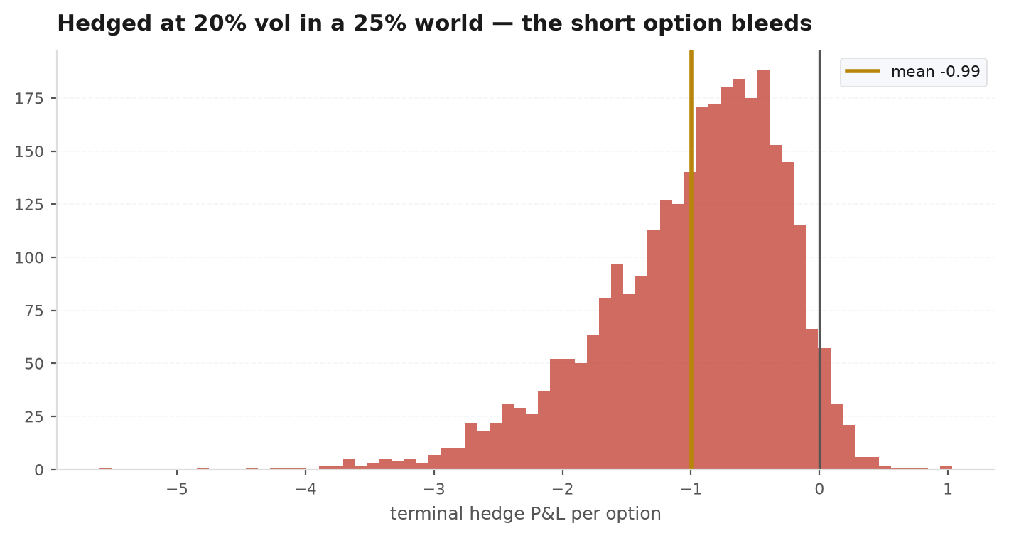
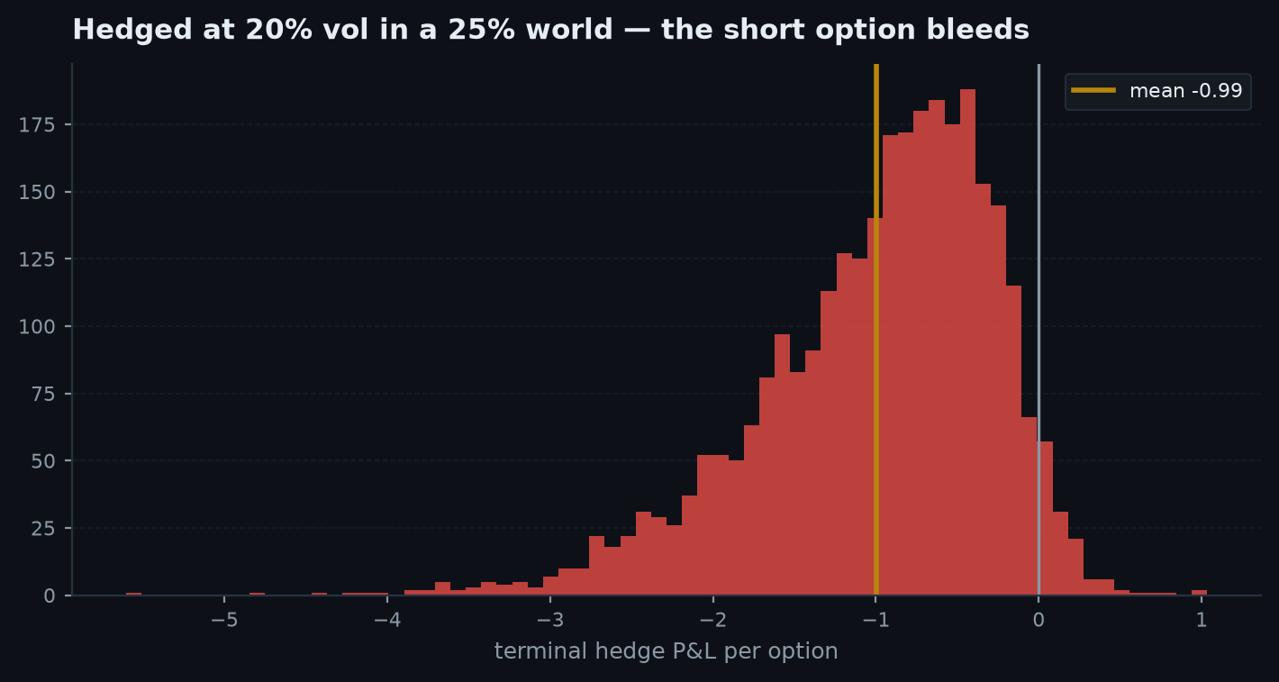
sim["pnl"]    # full distribution across paths — plot it

✦Scenario — the hedging-error histogram when realized beats implied

Run the block above: short a 1-year ATM call sold at $20%$ implied, hedged weekly (52 steps), in a world realizing $30%$ . The identity predicts the mean loss — integrate $\frac{1}{2} Γ S^{2} (σ_{real}^{2} - σ_{imp}^{2})$ over the year, or shortcut it with vega: an ATM 1-year call has vega $\approx 0.4 S T / 2 π \approx $0.40$ per vol point on $S_{0} = $100$ , so ten points of vol gap costs the seller roughly $$4$ per option. The simulation prints $mean \approx - $4.1$ , $std \approx $2.3$ . Note what the histogram says: with weekly hedging, a ten-vol-point edge is only $\approx 1.8$ standard deviations — around 4% of paths the seller profits despite being wrong about vol, because the paths happened to wiggle where gamma was small. Hedge daily and the noise drops by $5$ to $\approx $1.0$ , and the vol gap dominates. Discreteness is why vol P&L must be judged as a distribution — over many paths or many months — never one trade at a time.

Histogram of delta-hedging P&L across simulated paths, centred on the negative vol-gap mean with dispersion from discrete rebalancing — P&L distribution for the short-a-20-vol-call-in-a-30-vol-world hedger, 52 rebalances. The centre of mass is the vol-gap loss the identity predicts; the spread is discrete-hedging noise, shrinking like 1/sqrt(n) as rebalancing gets finer. The right tail shows the sobering part: being right about vol does not guarantee winning on any single path.

!The surface is a consensus, not a truth

Realized-vs-implied is a statistical edge with the payoff shape of insurance dealing: selling rich vol wins steadily until the tail arrives — the same negative skew as carry, and the same sizing discipline applies. And the smile’s “overpricing” of wings is partly real risk premium for jumps the diffusion identity above cannot see. Before trading any surface signal, put it through the gauntlet with the tail explicitly stressed.

Next: every trade in this part — factor rebalances, event entries, carry rolls, hedge adjustments — must actually be executed, and execution has a price. How to trade a position into existence without paying away the edge: Optimal execution.