Why most backtests lie

A beautiful equity curve is the easiest thing in the world to produce and one of the least meaningful. This chapter is the hinge of the whole course: it shows, with math, exactly how a backtest fools you — noise mistaken for signal, the same data mined until something shines, the best of many random tries dressed up as a discovery. Understanding this is what makes the testing chapters that follow feel necessary rather than pedantic.

Noise vs signal#

Every price series is part signal (a real, repeatable relationship) and mostly noise (random fluctuation that will never repeat). A backtest cannot tell you which is which — it faithfully reports the performance of whatever pattern you fit, real or imaginary. The trouble is that noise is structured enough to look like signal over any finite sample. Given a few hundred bars, you can always find a rule that would have traded them beautifully; the question is whether that rule describes the market or just that particular slice of history.

The cruel asymmetry: a real edge is small and noisy (recall the standard error from Statistics for traders), while an over-fit rule looks clean and large. So the more impressive a backtest looks, the more suspicious you should be — real edges are usually thin and ugly.

Data mining & p-hacking#

Data mining is searching the same dataset for a pattern that works; p-hacking is doing it until something clears a significance bar. Both exploit a loophole in the p-value from earlier: a p-value is only valid for a single, pre-registered test. Try many, and you have quietly changed the experiment.

Every knob is a hidden test. Sweeping a lookback from 10 to 200, trying five stop multiples, three targets, and four instruments is $191 \times 5 \times 3 \times 4 = 11, 460$ strategies. Report the best one’s p-value as if you had run one test and you are lying to yourself with arithmetic. This is the most common way honest people produce dishonest backtests.

The multiple-testing problem#

Here is the math that should scare you. If you run $N$ independent tests on pure noise, each with a false-positive rate $α$ , the probability that at least onecomes up “significant” is:

P (at least one false positive) = 1 - (1 - α)^{N}

✦Derivation — the complement of 'no false positives'

Work with the complement. Under the null (pure noise), one test is a false positive with probability $α$ , so it is not a false positive with probability $1 - α$ . If the $N$ tests are independent, the probability that all of them clear (no false positive anywhere) is the product $(1 - α)^{N}$ . “At least one false positive” is the complement of “none,” so

FWER = P (\geq 1 false positive) = 1 - P (none) = 1 - (1 - α)^{N} .

Bonferroni correction. To hold the family-wise error at $α$ across $N$ tests, test each at the stricter threshold $α / N$ . The guarantee needs no independence — it follows from Boole’s union bound, $P (⋃_{i} A_{i}) \leq \sum_{i} P (A_{i})$ :

FWER = P (⋃_{i = 1}^{N} {test i false-pos}) \leq i = 1 \sum N \frac{α}{N} = α .

Why it matters for trading. Every knob you sweep is a hidden test, so your effective $N$ is enormous and the honest per-config threshold is brutal. The best config in an 11,460-strategy sweep must clear roughly $0.05/11, 460 \approx 4 \times 1 0^{- 6}$ , not $0.05$ , before its p-value means anything.

At $α = 0.05$ , just 14 tests give you better-than-even odds of a spurious winner; at 100 tests it is 99.4% certain. You will find a $p < 0.05$ strategy in random data if you look at enough of them — guaranteed.

✦Scenario: sweeping SmaCross into a fake winner

You optimise a plain SmaCross: fast MA over

{5, 10, \dots, 50}

(10 values), slow MA over

{60, 80, \dots, 200}

(8 values), across 4 instruments —

10 \times 8 \times 4 = 320

backtests. Even if none of these has a real edge, at

α = 0.05

you expect

320 \times 0.05 = 16

of them to clear “

p < 0.05

” by luck alone, and the very best might post a profit factor near 1.6 with a gorgeous curve. Report thatone as if it were your single idea and you have p-hacked without meaning to. The honest bar is not 0.05 but Bonferroni’s

0.05/320 \approx 1.6 \times 1 0^{- 4}

— and the real defense is to hold out data the sweep never touched and see if the winner repeats.

The expected maximum of N random strategies#

It gets worse: not only will one clear the bar, the best of your random tries will look genuinely spectacular. If you generate $N$ strategies with no real edge — each a standard Normal Sharpe — the expected value of the maximum grows without bound as you add more:

E [1 \leq i \leq N max Z_{i}] \approx 2 ln N

→Sketch — where √(2 ln N) comes from

The maximum sits near the level $t$ that you expect to be exceeded about once in $N$ draws — i.e. where $N P (Z > t) \approx 1$ . For a standard Normal the upper tail decays like $P (Z > t) \approx \frac{1}{t 2 π} e^{- t^{2} /2}$ . Keeping the dominant exponential factor, set

N e^{- t^{2} /2} \approx 1 \Rightarrow \frac{t ^{2}}{2} \approx ln N \Rightarrow t \approx 2 ln N .

The maximum of $N$ iid standard Normals concentrates tightly around this level (extreme-value theory sharpens it to $2 ln N - \frac{l n l n N + l n 4 π}{2 2 l n N}$ , but the leading term is what bites). Why it matters for trading: a Sharpe estimate is approximately Normal around its true value, so the best of $N$ edge-free strategies has an expected Sharpe of about $2 ln N$ standard errors above zero purely from selection. Growing the search only makes the winner look better while its true edge stays exactly zero — best-of-N noise is indistinguishable from skill until you test out-of-sample.

Test 1,000 worthless strategies and the best one has an expected Sharpe around $2 ln 1000 \approx 3.7$ standard errors from zero — a “3-sigma discovery” that is pure selection. The winner of a large search is not the one with an edge; it is the one that got luckiest. Its out-of-sample performance regresses straight back to zero.

The best Sharpe found among N random strategies rising with the number of strategies tested — Best-of-N on pure noise: the maximum Sharpe among N edge-free strategies climbs like √(2 ln N). A 'great' backtest selected from a large search is expected even when nothing works — the winner is the luckiest, not the best.

✕The best backtest you ran is the one you should trust least

Selection is not a minor caveat — it is the dominant force in any strategy search. The very act of picking the top performer biases its metrics upward. Any honest evaluation must penalise for how many things you tried.

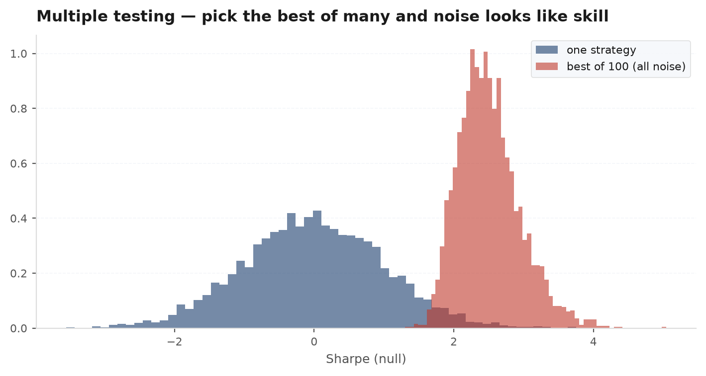
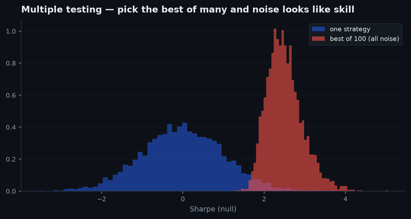
This is why edgekit’s validation layer carries a deflated_sharpe — a Sharpe adjusted down for the number of trials it took to find the winner — precisely to undo the $2 ln N$ inflation.

deflated.py

from edgekit.validation import deflated_sharpe

# You searched ~200 configs and kept the best. Its raw Sharpe is inflated
# by that selection — deflate it against the number of trials.
ds = deflated_sharpe(winning_returns, n_trials=200, sr_std=0.03)
print(ds)   # a Sharpe that survives this is one selection didn't manufacture

The base-rate fallacy — the most important lesson in the chapter#

A significant p-value answers $P (significant ∣ no edge)$ — the chance noise fakes your result. But the question you actually care about is the reverse: $P (real edge ∣ significant)$ — given that my backtest cleared the bar, how likely is the edge real? These are not the same number, and confusing them is the base-rate fallacy. Bayes’ theorem converts one into the other:

P (real ∣ sig) = \frac{P ( sig ∣ real ) P ( real )}{P ( sig )}, P (sig) = P (sig ∣ real) P (real) + P (sig ∣ fake) P (fake) .

The term $P (real)$ is the prior base rate — the fraction of strategies you try that have a genuine edge — and it is low. Real edges are rare; most ideas are variations on noise. Plug in a sober prior $P (real) = 0.05$ , a test with power $P (sig ∣ real) = 0.80$ , and the usual false-positive rate $P (sig ∣ fake) = 0.05$ :

P (real ∣ sig) = \frac{0.80 \times 0.05}{0.80 \times 0.05 + 0.05 \times 0.95} = \frac{0.040}{0.040 + 0.0475} = \frac{0.040}{0.0875} \approx 0.46.

Read that again: even a correctly significant, $p < 0.05$ backtest is more likely false than true — a 54% chance the “edge” is noise — before you account for any data mining. And multiple testing makes it strictly worse: searching many configs inflates the effective $P (sig ∣ fake)$ far above 0.05 (that is what the $1 - (1 - α)^{N}$ result above measures), so the denominator balloons and the posterior collapses toward zero.

!Why it matters for trading — this is the whole game

You cannot raise a low posterior by staring harder at the same p-value; the only levers are the prior and the false-positive rate. That is exactly what good process does: a sound economic rationale raises

P (real)

before you test, and out-of-sample validation, permutation, and cost stress drive

P (sig ∣ fake)

down. A significant backtest is the start of the argument, never the end of it.

Overfitting, formalised#

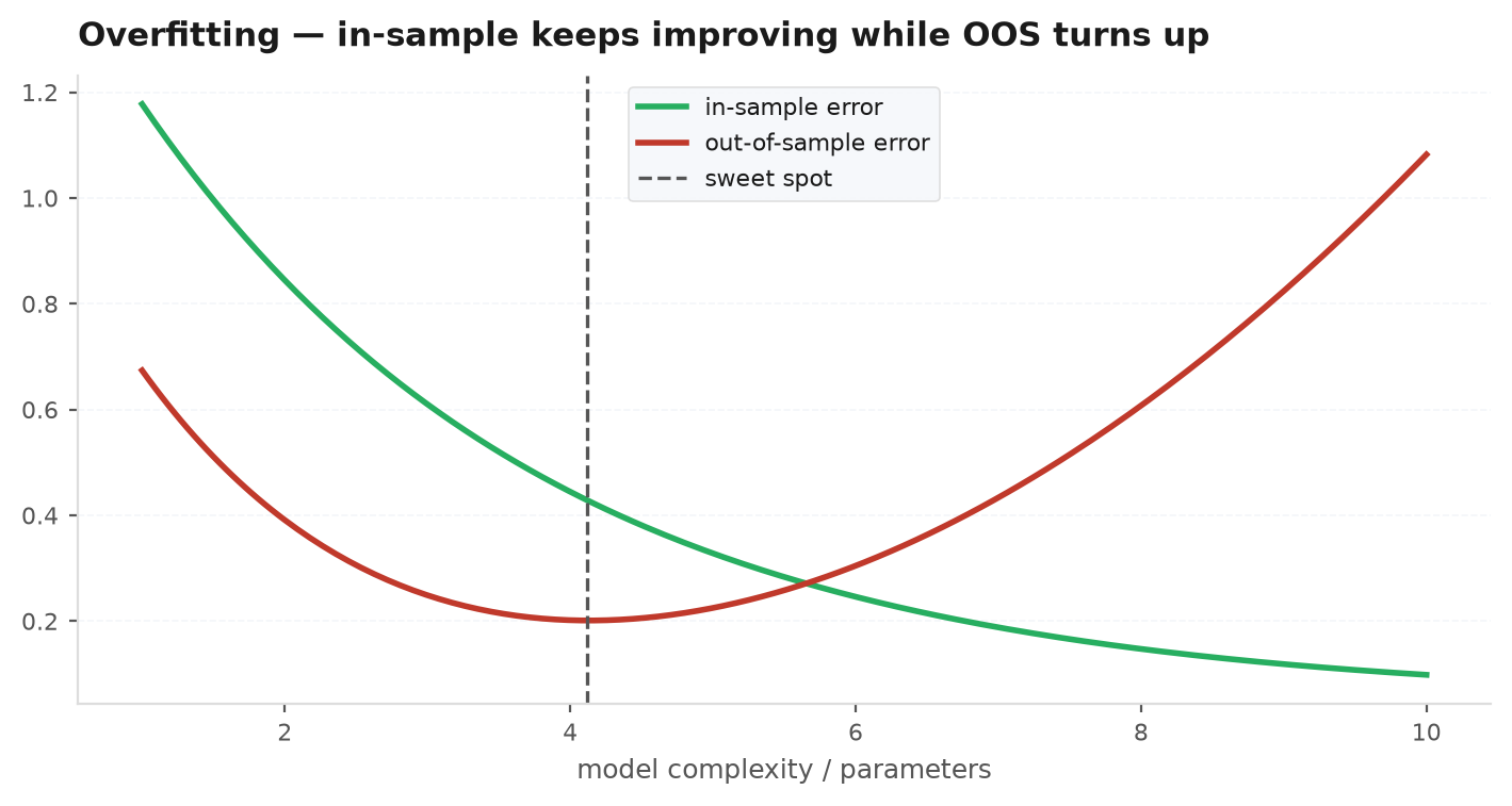
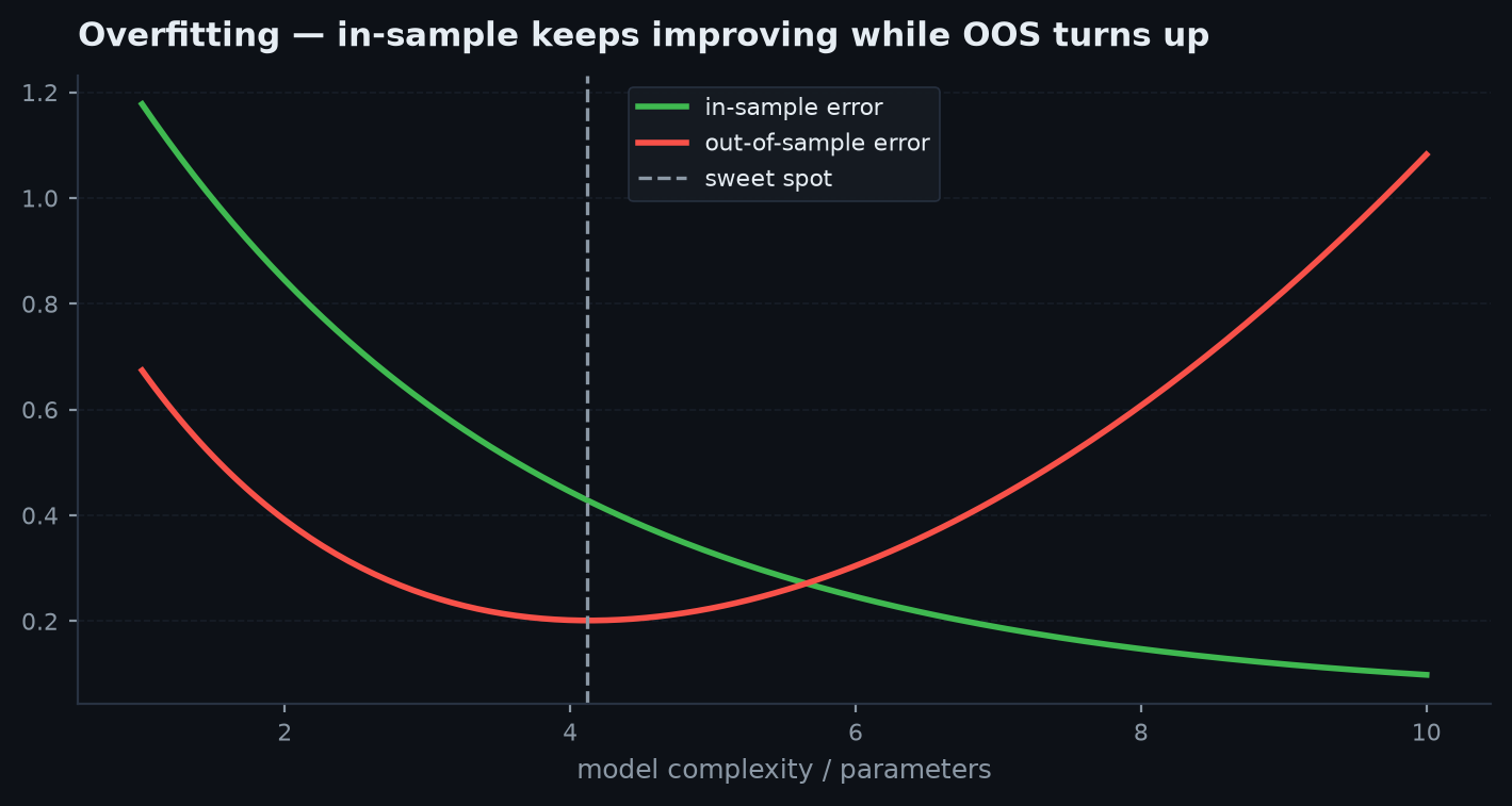
Overfitting is fitting the noise instead of the signal. Any model flexible enough will drive its in-sample error toward zero by memorising the particular wiggles of the training data — wiggles that carry no information about the future. The tell is a widening gap between in-sample and out-of-sample performance:

Generalization gap = what you’ll actually get Error_{out-of-sample} - what the backtest showed Error_{in-sample}

→Why the in-sample number is optimistic by construction

When you choose parameters $θ$ to minimiseerror on the training sample, you are optimising against that sample’s particular noise as well as its signal. Decompose an estimator’s expected error into bias, variance, and irreducible noise:

E [(y^- y)^{2}] = too-simple (bias)^{2} + fits noise variance + irreducible σ^{2} .

Adding complexity buys lower bias but higher variance — and variance is the part that does not transfer to new data. In-sample error keeps falling because the fit absorbs both terms; out-of-sample error can only fall until the variance term overtakes the bias saving, then it rises. Why it matters for trading: the gap is not measurable from the backtest alone — the training curve always looks good — which is exactly why you must hold out unseen data (walk-forward) to estimate it rather than assume it away. See Overfitting detection.

✦Scenario: the ten-knob strategy that only knew 2021

A colleague shows you a BTC strategy with ten hand-tuned rules — a lookback of 37, a stop at 2.3 ATR, a volume filter above 1.8×, a “skip Mondays” toggle, and so on — with a flawless 2021 equity curve and a Sharpe near 3. Each oddly-specific knob was chosen because it improved that year’s backtest, which means the knobs are describing 2021’s particularnoise: the exact chop, the exact rallies. Run it untouched on 2022 and it falls apart — Sharpe goes negative — because 2022’s noise is different noise. The in-sample number was never a forecast; it was a memory. That gap between the beautiful 2021 curve and the ugly 2022 one is the generalization gap made visible, and the ten degrees of freedom are exactly what bought it.

As you add parameters or search harder, in-sample error keeps falling but out-of-sample error turns around and rises — the model has started describing this history rather than the market. The sweet spot is well before the in-sample minimum; past it you are buying backtest beauty with live losses.

In-sample error falling while out-of-sample error falls then rises with model complexity — The overfitting curve. In-sample error (lower line) falls monotonically with complexity; out-of-sample error (upper line) bottoms out then climbs. The gap between them is overfitting — and the backtest only ever shows you the lower line.

!Degrees of freedom are a budget you are spending

Every parameter, filter, and hand-tuned threshold is a degree of freedom spent fitting the past. A strategy with two robust rules that works everywhere beats one with ten finely-tuned knobs that works only on the data it was born from. Simplicity is not aesthetics — it is out-of-sample insurance.

Regime dependence#

Even a genuinely-fit strategy carries a hidden assumption: that the future resembles the past. Markets move through regimes— trending vs ranging, calm vs volatile, low-rate vs high-rate — and an edge that was real in one regime can vanish or invert in the next. A backtest spanning a single long bull market can look flawless and be measuring nothing but that regime’s tailwind (the difference between alpha and beta, covered in Alpha vs beta).

The defense is to insist an edge holds across regimes, not just on average. Split the history — bull vs bear, high-vol vs low-vol — and demand the edge survive each slice, not merely the blended whole. A result that only appears when you pool everything together is a regime artifact wearing an edge’s clothing.

Regression to the mean & survivorship bias#

Selection has a quantitative signature. Write any measured performance as truth plus noise, $X = μ + ε$ , where $μ$ is the strategy’s real skill and $ε$ is sampling luck. When you pick the top result of a search, you preferentially pick strategies whose $ε$ was large and positive — so the winner’s luck is, on average, positive, and its future performance regresses toward the mean. The best linear estimate of the truth given the observation shrinks it toward the population average $μ ˉ$ :

E [μ ∣ X] = μ ˉ + ρ (X - μ ˉ), ρ = \frac{σ _{μ}^{2}}{σ _{μ}^{2} + σ _{ε}^{2}} < 1.

The reliability $ρ$ is the share of observed variance that is real signal. When noise dominates $(σ_{ε}^{2} ≫ σ_{μ}^{2})$ , $ρ \to 0$ and your best forecast of a chart-topping backtest’s future is the average — near zero edge. This is regression to the mean stated as an equation, and it is the deep reason out-of-sample numbers come in below in-sample ones.

Survivorship bias is the same conditioning applied by the world instead of by you. The strategies, funds, and coins you can study are the ones that survived; the failures were delisted and deleted. Conditioning on survival lifts the observed mean above the true mean, $E [return ∣ survived] > E [return]$ , so a backtest on today’s tradable universe is quietly scored on a sample hand-picked for having done well.

!Why it matters for trading

Both effects push the same direction — your live results will, on average, come in below your best backtest — and neither is a bug you can fix by trying harder. The only defenses are to shrink extreme estimates before you trust them (deflated Sharpe does this) and to test on data and instruments that were not pre-selected for success (walk-forward, point-in-time universes).

This is why the gauntlet exists#

Every failure above has the same shape — a result that looks real in-sample and dies out-of-sample — and each has a specific antidote. Stacked together, they are the gauntlet:

The lie	The defense	Where in edgekit
Noise mistaken for signal	Permutation test — could shuffled data fake this?	`validation.mcpt`
Best-of-N selection inflation	Deflated Sharpe — penalise for trials	`validation.deflated_sharpe`
Overfitting to one period	Walk-forward — test on unseen data	`validation.walk_forward`
Regime dependence	Regime splits — demand edge in each	the gauntlet
One lucky historical path	Monte Carlo — resample the outcome	Monte Carlo
Costs quietly ignored	Cost stress — 2× the fees, does it live?	`costs.cost_stress`

✦The mindset to carry forward

Treat every backtest as guilty until proven innocent. Your job is not to build a strategy that looks good — that is trivial — but to try to kill a strategy and report the ones that refuse to die. The illustrativeORB and SmaCross strategies in edgekit are here to practice that adversarial process, and most of them do not survive it. That is the point.

Next: with the math of edge and the ways it deceives us in hand, Part III turns to building — starting with the Anatomy of a strategy. The defenses named above are built out in full in Part IV, beginning with Backtesting fundamentals.