Cross-sectional factor investing

Everything so far predicted one series through time: will this asset go up tomorrow? This chapter rotates the problem ninety degrees. Cross-sectional investing asks a different question at each date: of these hundred assets, which oneswill beat the others? The tools change with the question — portfolio sorts replace signal thresholds, and the Fama–MacBeth two-pass regression replaces the single time-series fit — but the statistical skepticism of the gauntlet transfers intact.

✦Intuition — the pivot from timing to ranking

A time-series trader needs to know whether Bitcoin rises next week — a hard, low-signal call on one noisy series. A cross-sectional trader never makes that call. They rank 100 stocks by some characteristic — last year’s return, cheapness, profitability — buy the top slice, short the bottom slice, and let the market leg cancel out. Whether the whole market rises or crashes is (to first order) irrelevant: the bet is purely that the ranking carries information about relative returns. That is a statistically easier game: instead of one observation per period you get a whole cross-section of them, and instead of predicting a level you only need to predict an ordering. The price of admission is a new inference machinery — because now the noise is correlated across assets within each period, and naive t-stats lie.

Time-series vs cross-sectional prediction#

Formally, a time-series signal is a map from an asset’s own history to its expected return, $E [r_{i, t + 1} ∣ F_{i, t}]$ . A cross-sectional signal is a characteristic $z_{i, t}$ — one number per asset per date — that predicts returns relative to the cross-sectional average:

E [r_{i, t + 1} - r ˉ_{t + 1} ∣ z_{i, t}] = λ z_{i, t} .

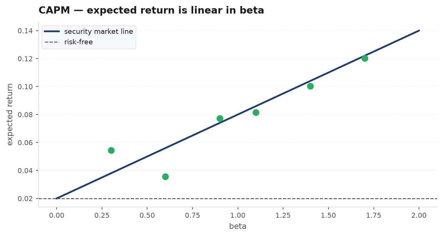
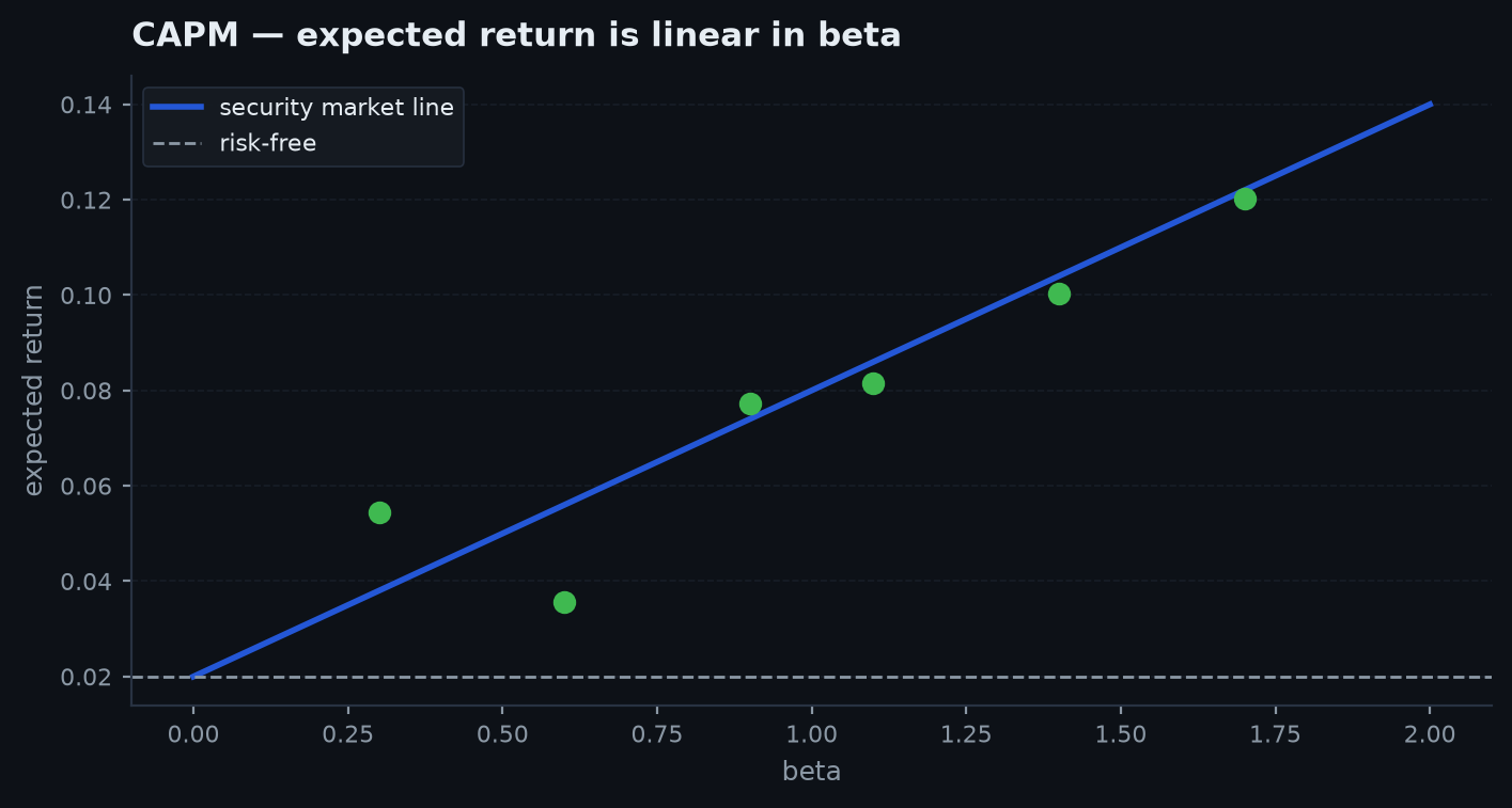
The coefficient $λ$ is the factor premium: the extra return earned per unit of the characteristic. A long-short portfolio built from the ranking earns $λ$ times the spread in $z$ it holds, with the market component differenced away. This is the same alpha-vs-beta split as regression & factor models — but run across assets at a fixed daterather than across dates for a fixed asset. The CAPM’s security market line was already a cross-sectional prediction: expected return linear in beta, across assets.

The security market line: expected excess return against beta across assets, the original cross-sectional prediction — The security market line, revisited. CAPM's claim was always cross-sectional: at any date, expected excess returns across assets should line up against their betas. Factor investing generalises the x-axis — replace beta with momentum, value, quality — and tests whether the slope (the premium) is reliably nonzero.

Portfolio sorts: deciles and the long-short spread#

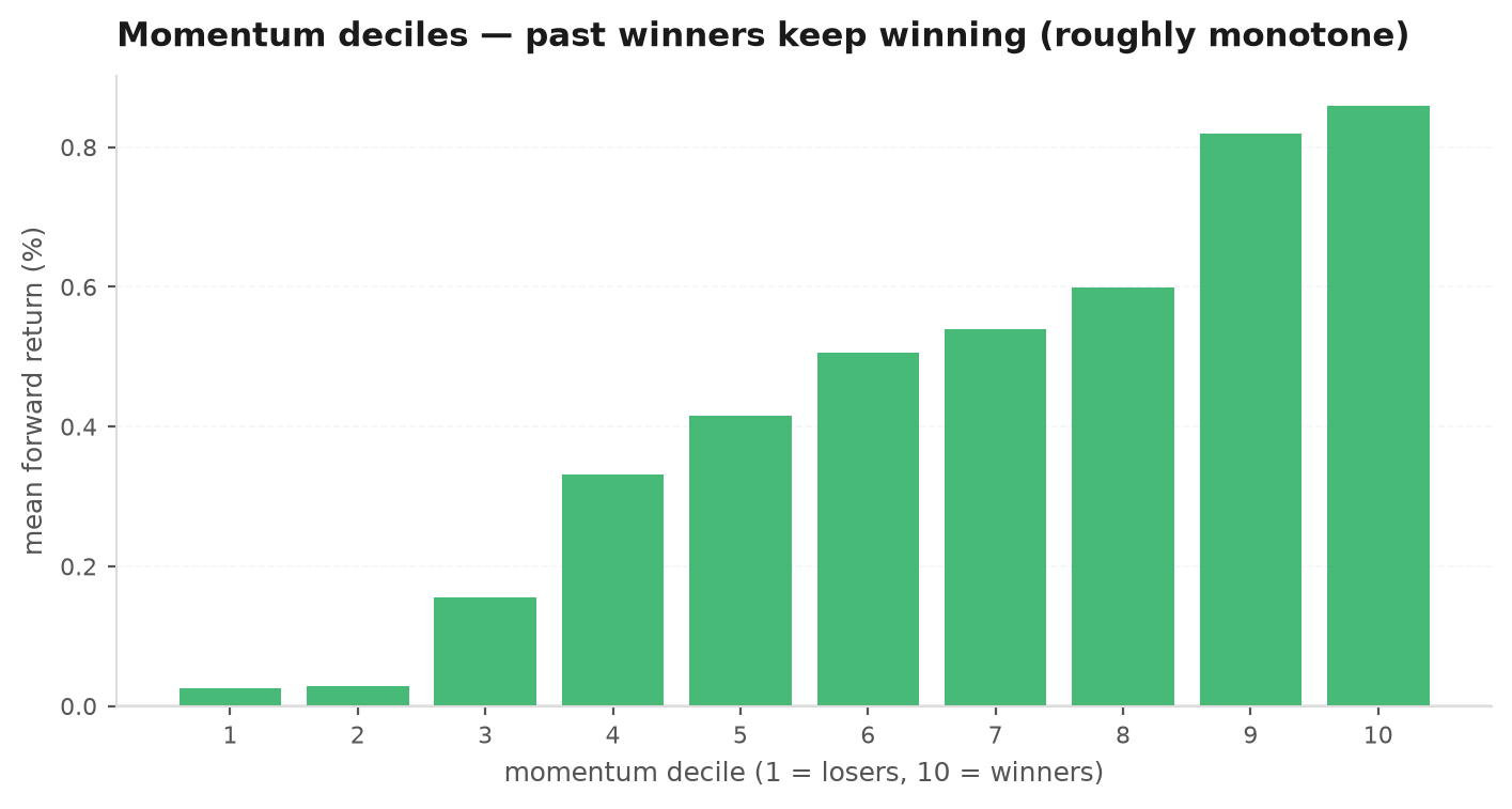
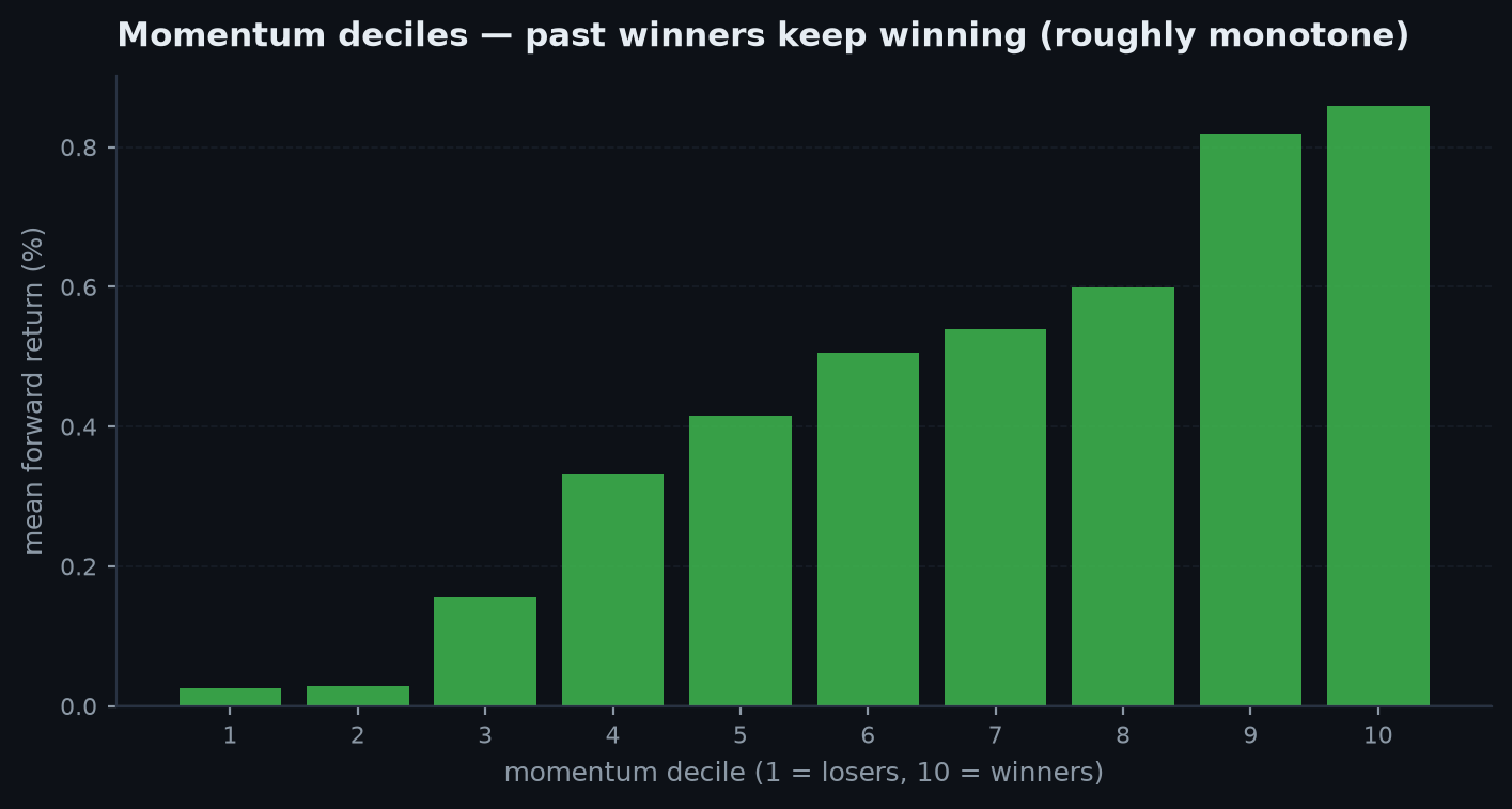
The workhorse test is embarrassingly simple. At each rebalance date, rank all assets by the characteristic, split them into deciles (D1 = lowest, D10 = highest), and hold each decile as an equal-weight portfolio until the next rebalance. If the characteristic prices the cross-section, average returns should rise monotonically across deciles, and the long-short spread

r_{t}^{LS} = r_{t}^{D 10} - r_{t}^{D 1}

should have a positive mean. The spread portfolio is (roughly) market-neutral by construction — both legs hold the same market exposure with opposite signs — so its mean is a direct estimate of the premium, uncontaminated by whether the index happened to rally over the sample.

Bar chart of average monthly return for ten momentum-sorted decile portfolios, rising from losers on the left to winners on the right, with the D10 minus D1 spread highlighted — Momentum decile portfolios. Assets are ranked each month by their 12-1 past return and grouped into deciles; the bars are each decile's average forward return. A monotone staircase is the signature of a real cross-sectional signal — and the D10 − D1 spread on the right is the long-short premium a factor portfolio harvests.

→Why sorts before regressions

A sort makes no functional-form assumption: if the characteristic predicts returns in any monotone way, the decile staircase shows it. It is also the honest first look at implementability — a premium that lives entirely in D1 (shorting illiquid losers) is a very different trade from one spread evenly across the ranking. Regressions come second, to attach standard errors and control for other characteristics.

The factor zoo#

Four families of characteristics have survived decades of out-of-sample scrutiny — and hundreds more have been published and quietly died. The survivors:

Momentum— the return from twelve months ago to one month ago (the “12-1” convention skips the last month, which reverses). Winners keep winning for 3–12 months. The premium is strong but crashes violently when the market snaps back (momentum is short the rebound).
Value — cheap on fundamentals (book-to-market, earnings yield) beats expensive. Slow-moving, decade-scale cycles; the natural diversifier to momentum (their correlation is negative).
Quality — profitable, low-accrual, conservatively financed firms beat junk. The premium is modest but stable, and pays most in downturns.
Low volatility — boring low-beta assets earn more per unit of risk than the SML says they should (the flat-SML anomaly), plausibly because leverage-constrained investors overpay for lottery-like high-beta names.

Fama–MacBeth: the two-pass regression#

Sorts show a premium; Fama–MacBeth measures it with standard errors that respect the panel structure. The insight: run one cross-sectional regression per period, then treat the sequence of estimated slopes as a time series and test its mean.

✦Derivation — period-by-period OLS, then average the slopes

Pass 1 (each period). At each date $t$ , regress the $N$ realised returns on the lagged characteristics across assets:

r_{i, t} = λ_{0, t} + λ_{t} z_{i, t - 1} + ε_{i, t}, i = 1, \dots, N,

giving one slope estimate $λ^_{t}$ per period — the realised reward, that period, for holding a unit of the characteristic. Pass 2 (across periods). The premium is the time-average of the slopes, and — the elegant part — its standard error comes from the time-series dispersion of the estimates themselves:

λ^= \frac{1}{T} t = 1 \sum T λ^_{t}, se (λ^) = \frac{s _{λ^_{t}}}{T}, t_{FM} = \frac{λ ^}{se ( λ ^ )} .

Why this fixes the panel problem. A pooled regression on all $N \times T$ observations would count each period’s $N$ stocks as independent draws — but stocks move together within a period, so the effective sample size is closer to $T$ than $N \times T$ . Fama–MacBeth builds this in automatically: whatever cross-sectional correlation exists inside a period is swallowed into that period’s single $λ^_{t}$ , and the inference runs on $T$ honest observations. Each $λ^_{t}$ is also exactly the return of a tradable zero-cost portfolio with unit exposure to $z$ — the regression is a backtest in disguise.

Time series of period-by-period Fama-MacBeth slope estimates oscillating around a positive mean, with the time-average premium and its confidence band marked — The second pass, visualised. Each point is one period's cross-sectional slope — the realised premium that month. The premium estimate is the time-average of these noisy slopes; its standard error is their standard deviation over sqrt(T). The premium is 'real' when the band around the mean excludes zero.

Why Newey–West errors matter#

The $s_{λ^_{t}} / T$ formula assumes the period slopes are serially uncorrelated. They rarely are: premia trend and crash (momentum especially), characteristics overlap across formation windows, and volatility clusters. Positive autocorrelation makes the naive standard error too small — the same disease that afflicted plain OLS t-stats in regression & factor models. The repair is the Newey–West (HAC) estimator, which inflates the variance of the mean with a weighted sum of autocovariances:

Var (λ^) = \frac{1}{T} [γ^_{0} + 2 ℓ = 1 \sum L (1 - \frac{ℓ}{L + 1}) γ^_{ℓ}],

where $γ^_{ℓ}$ is the lag- $ℓ$ autocovariance of the $λ^_{t}$ series and the Bartlett weights keep the estimate positive. edgekit’s ek.factors.fama_macbethreports Newey–West t-stats by default; ek.factors.newey_west exposes the HAC standard error of any mean directly.

fama_macbeth.py

import edgekit as ek

# returns: T×N DataFrame of asset returns
# mom:     T×N DataFrame of the 12-1 momentum characteristic,
#          ALREADY lagged — row t must be knowable before period t's return
fm = ek.factors.fama_macbeth(returns, {"momentum": mom})

fm["premia"]      # time-average slope per characteristic (the premium)
fm["t_nw"]        # Newey-West t-stat on each premium
fm["by_period"]   # the full T-length series of period slopes

# the HAC machinery on its own — se of the mean of any series:
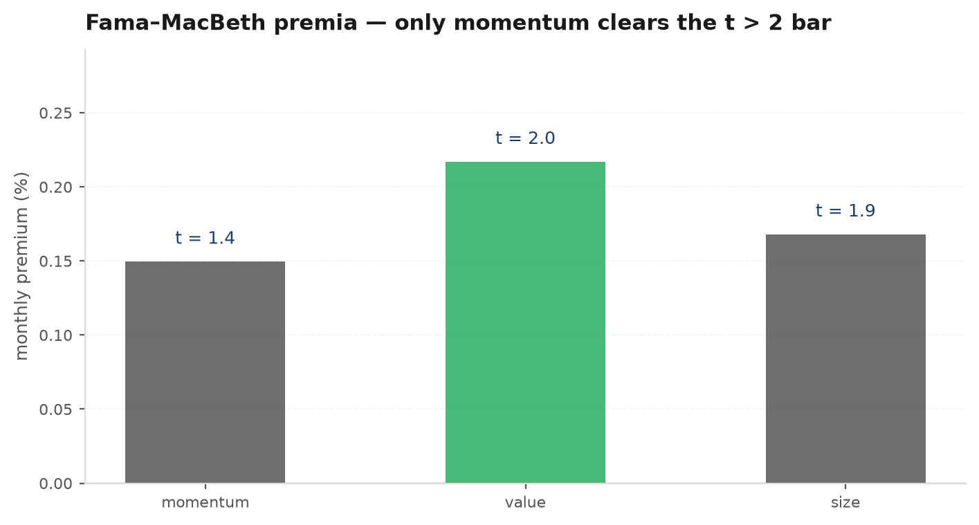
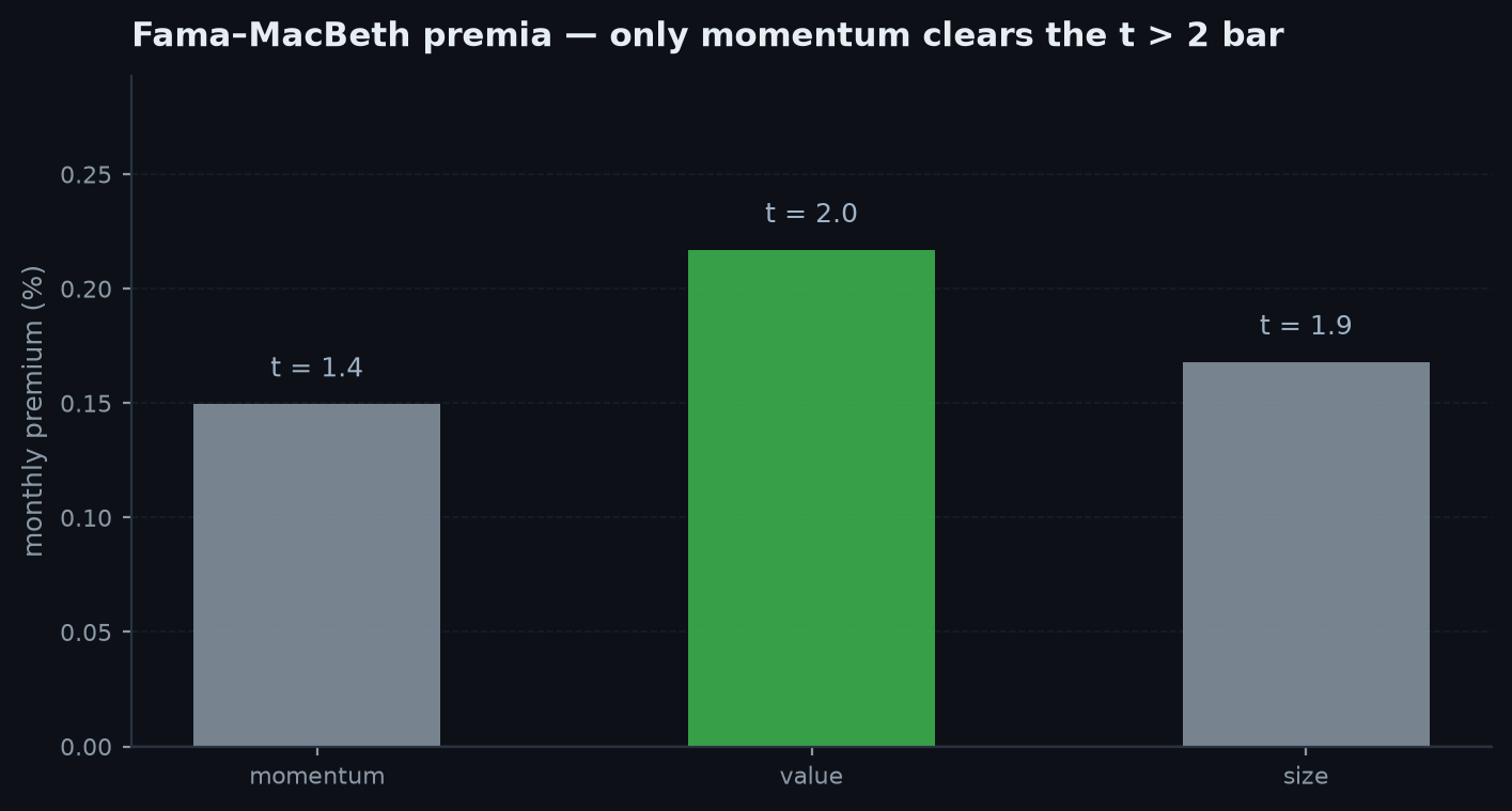
se = ek.factors.newey_west(fm["by_period"]["momentum"], lags=6)

✦Scenario — 12-1 momentum on a 100-stock panel

Take 100 stocks, 60 months. Each month, rank by the 12-1 return, form deciles, and record forward returns. Suppose the sort delivers D10 averaging $1.6%$ /month and D1 averaging $0.2%$ /month — a long-short spread of $1.4%$ /month, roughly $18%$ /year before costs. Now the inference. Fama–MacBeth on the standardised characteristic gives period slopes averaging $λ^= 0.90%$ with a standard deviation of $3.4%$ across the 60 months:

se = \frac{3.4%}{60} = 0.44%, t_{FM} = \frac{0.90}{0.44} \approx 2.05.

Just significant. But the slope series has lag-1 autocorrelation of $0.2$ — momentum premia trend — and Newey–West with 6 lags inflates the standard error to $0.53%$ , dragging the t-stat to $1.7$ . The premium is plausible but unproven on this sample: sixty months is simply not much evidence about a noisy, autocorrelated premium, no matter how wide the panel is. That is the recurring lesson of the two-pass logic — the cross-section buys you precision within a period, but the number of periods still governs what you can claim.

The tradable version is ek.strategy.CsMomentum: rank on the lagged 12-1 return, long the top fraction, short the bottom, rebalance monthly, with all weights shifted so no future information leaks in.

cs_momentum.py

import edgekit as ek

strat = ek.strategy.CsMomentum(lookback=126, skip=21,
                               top_frac=0.2, rebalance="ME")
out = strat.backtest(prices)        # prices: T×N DataFrame

out["weights"]   # T×N weights, causal (shifted after formation)
out["returns"]   # long-short portfolio return series

# then treat it like any strategy: gauntlet first, sizing second
sr = ek.metrics.sharpe(out["returns"], periods_per_year=252)

Data-snooping in the factor zoo#

Hundreds of published factors, thousands of unpublished ones — and every one of them was found by researchers running sorts and Fama–MacBeth regressions on largely the same historical panel. That is a textbook multiple-testing problem: test 300 candidate characteristics at the $∣ t ∣ > 2$ bar and you expect a dozen “discoveries” from pure noise.

Claim	The snooping failure mode	Defence
A new factor works	300 candidates tested, winners published	Raise the bar: \|t\| > 3, not 2 (see multiple testing)
Premium is stable	Formation window tuned in-sample	Out-of-sample and post-publication data only
Spread is tradable	D1 leg lives in illiquid micro-caps	Cost model + capacity check before believing it
Factor is 'new'	Correlated 0.9 with value or momentum	Regress it on the survivors; test the residual

!The zoo is a graveyard with good marketing

Most published premia shrink by half or vanish outright after publication — part arbitrage, mostly snooping. Treat a factor exactly like a backtest: the historical t-stat is the start of the argument, not the end. Apply the deflated bars from multiple testing and the full skepticism of why backtests lie — a cross-section of 100 assets multiplies your data, but it multiplies your ways to fool yourself just as fast.

Next:cross-sectional logic asks “which asset”; the event study asks “what happens after a defined trigger” — and how to test it without fooling yourself. Event studies & seasonality.