Carry & term structure

Trend bets that prices keep moving; mean-reversion bets that they come back. Carry is the third great return source, and it needs no price forecast at all: it is what you earn if the price does nothing — the bond coupon, the interest-rate differential, the futures roll, the perp funding payment. This chapter derives carry from the futures term structure, tours its FX and crypto incarnations, and confronts the catch that defines the trade: carry pays you steadily for insuring against a crash that eventually happens.

✦Intuition — the return of a frozen world

Take any position and ask: if every spot price in the world were frozen for a year, what would I earn? A bond still pays its coupon. A high-yield currency funded by a low-yield one still collects the rate gap. A futures contract still slides along its curve toward spot as expiry approaches. A short perpetual still receives its funding every eight hours. That frozen-world return is carry. It is visible in advance— printed in today’s prices and rates, no forecasting model required — which is exactly what makes it seductive: it feels like arbitrage. It is not. The market pays visible carry as compensation for an invisible risk, and the whole craft of carry trading is pricing that risk honestly.

The third return source#

It helps to place carry against the two return sources the earlier chapters built. Each answers a different question about the same price series:

Trend bets on continuation — that a move already underway persists. It needs the price to keep moving; it earns nothing (and bleeds costs) in a flat market.
Mean-reversion bets on a stretched price snapping back toward an anchor. It needs the price to move back; a market that trends away from the anchor is its nightmare.
Carry bets on nothing moving at all. Its return is contractual — a rate gap, a curve slope, a funding payment — realised so long as spot behaves. Its nightmare is the violent repricing that arrives precisely because so many others are harvesting the same payment.

The three are close to orthogonal by construction — they condition on different states of the world — which is why serious books run all three. But orthogonal in normal timesis the operative phrase; the crash state is where carry’s correlations misbehave, and this chapter keeps returning to it.

The futures term structure#

A futures curve plots, at one instant, the prices of contracts on the same underlying across delivery dates $T$ . Its shape has names:

Contango — the curve slopes up: deferred contracts cost more than spot. Typical when storage is costly and convenience yield is low (gold, calm oil markets, VIX futures most of the time).
Backwardation — the curve slopes down: deferred contracts are cheaper than spot. Typical when holding the physical asset now is valuable (supply squeezes, high convenience yield).

The shape is not a forecast of where spot is going — under no-arbitrage it is pinned by the economics of holding the underlying between now and delivery, the cost of carry:

F (T) = S e^{(r + c - y) T},

with financing rate $r$ , storage cost $c$ , and convenience (or dividend) yield $y$ . When $r + c > y$ the curve is in contango; when $y > r + c$ it is backwardated.

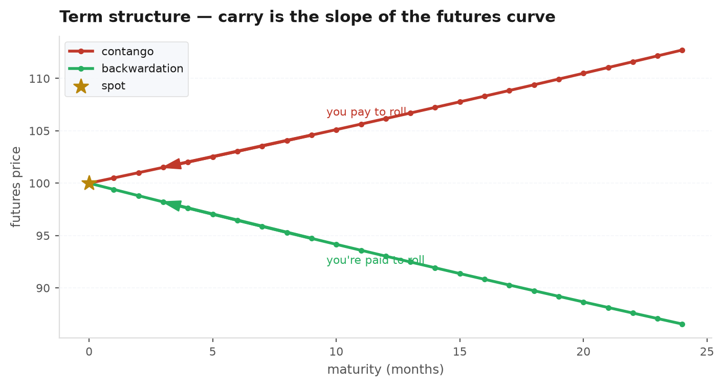
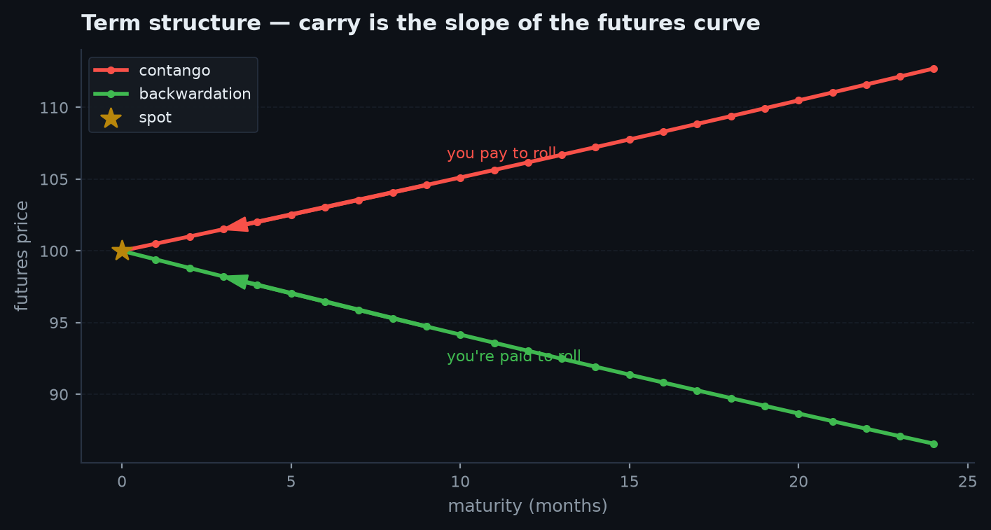
Two futures curves against time to delivery: an upward-sloping contango curve and a downward-sloping backwardated curve, converging to spot at zero — The futures term structure. Both curves are anchored at spot (T = 0). Contango slopes up — holding the future means buying dear and rolling down to spot, negative carry. Backwardation slopes down — the future is priced below spot and pulls up toward it, positive carry. The roll yield is the local slope of the curve.

✦Derivation — roll yield is the slope of the curve

Hold a futures contract while nothing happens: spot $S$ , rates, and the curve’s shape all stay frozen; only calendar time passes. Your contract’s time-to-delivery shrinks, so its price slides along the fixed curve toward spot. From the cost-of-carry formula, take logs and differentiate with respect to time-to-delivery:

ln F (T) = ln S + (r + c - y) T ⟹ \frac{d ln F}{d T} = r + c - y .

As the calendar advances, $T$ decreases, so the log-price of your contract changes at the rate

roll yield = - \frac{d ln F}{d T} = y - r - c .

Read it off the picture: the roll yield is minus the slope of the (log) futures curve. In backwardation the curve slopes down, so rolling up it toward spot earns positive carry; in contango you bleed the slope instead. This is the entire mechanical basis of futures carry strategies: rank markets by curve slope, be long the backwardated ones and short the contangoed ones — a cross-sectional sort where the characteristic is printed on the curve rather than estimated from history.

Numbers make the slope tangible. VIX futures spend most of their life in steep contango: a front-month contract 5% above spot VIX with one month to delivery rolls down at roughly $5%$ /month — a brutal $\approx 45%$ /yr headwind for naive long-vol ETPs, and the entire economic engine of the short-VIX products that compound it in reverse (until a vol spike deletes them). Crude oil in a supply squeeze can back-order to $1%$ /month of backwardation — a $12%$ /yr tailwind for the long. Same formula, opposite signs, and both printed on the curve before the trade is ever placed.

FX carry and the peso problem#

The oldest carry trade: borrow a low-yield currency (historically JPY), lend a high-yield one (AUD, BRL, TRY), and pocket the rate differential. The position’s log return decomposes into the contractual part and the price part:

r_{carry} = known in advance (i_{high} - i_{low}) Δ t + FX move, unknown Δ ln S .

Uncovered interest parity says the exchange rate should depreciate to eat exactly the differential — $E [Δ ln S] = - (i_{high} - i_{low}) Δ t$ — leaving zero expected return. Empirically it mostly does not — high-yield currencies have historically depreciated less than the differential implies, leaving positive average returns. The catch is the shape of those returns: years of small steady gains, then a violent unwind in which every crowded carry pair crashes at once (1998, 2008) as funding currencies spike and risk positions are cut simultaneously.

!The peso problem — averages estimated without the disaster

A sample that hasn’t yet contained the crash makes carry look like free money: the measured mean is biased up and the measured risk biased down, because the rare state that justifies the premium simply hasn’t been sampled. That is the peso problem, and it is why carry strategies must be judged by their tails, not their Sharpe. The right toolkit is extreme value theory: fit the tail explicitly, and size as if the crash year is in the data even when it isn’t.

Once you see the pattern — a visible payment for holding one thing against another — carry appears in every asset class, always with the same trade construction and the same skew:

Asset class	The carry	Where it's printed	The crash that pays for it
Bonds	Yield + rolldown along the curve	The yield curve	Rate spikes / curve inversion
FX	Interest-rate differential	Money-market rates	Funding-currency squeeze (1998, 2008)
Commodities	Roll yield	Futures curve slope	Curve flip on a supply shock
Equities	Dividend yield vs financing	Dividend futures, index basis	Dividend cuts in recessions
Crypto	Perp funding / futures basis	Funding prints every 8h	Liquidation cascades

Crypto carry: funding rates and the basis#

Crypto rebuilt the entire carry complex from scratch. A perpetual swap has no expiry, so exchanges tether it to spot with a funding rate: every 8 hours, if the perp trades above spot, longs pay shorts a fee proportional to the gap (and vice versa). Persistent speculative long demand keeps funding positive most of the time — meaning a hedged position (short perp, long spot) collects funding with no directional exposure. The dated-futures version is the basis trade: buy spot, short a future trading above it, and capture the annualised basis $(F - S) / S \cdot 1/ T$ as the two converge at expiry.

funding_carry.py

import edgekit as ek

# realised funding on the BTC perp (Binance, 8-hourly)
fr = ek.data.fetch_funding_rates("BTCUSDT", limit=1000)
ann = fr["rate"].mean() * 3 * 365          # annualised carry
print(f"avg funding: {ann:.1%}/yr")

# cross-sectional carry portfolio: long high-carry, short low-carry
strat = ek.strategy.Carry(top_frac=0.3, rebalance="W")
out = strat.backtest(prices, carry)        # both T×N DataFrames
out["returns"]                             # weekly long-short carry P&L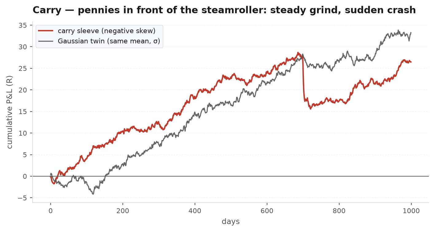

Cumulative P&L of a carry strategy: a long smooth upward grind punctuated by an abrupt deep drawdown, versus the steady line naive annualisation predicts — The signature carry equity curve: a smooth grind of collected funding, then a cliff. The strategy is short the crash — its return distribution is negatively skewed, so the mean return arrives with occasional violence. Naive annualisation of the calm stretch (dashed) is exactly the peso-problem estimate.

✦Scenario — 8%/yr of funding vs one crash week

A desk runs the hedged BTC trade: long $$1 M$ spot, short $$1 M$ perp. Funding averages $0.0073%$ per 8-hour interval — about $8%$ /yr — so the position drips in roughly $$219$ a day, $$80, 000$ a year, with near-zero price exposure. For ten months it does exactly that. Then a crash week: BTC drops $30%$ in days. The hedge holds — spot losses offset perp gains — but nothing else does: funding flips to $- 0.05%$ per interval (you now pay $\approx 55%$ /yr while unwinding), the exchange holding your short raises margin, the spot leg can’t be sold fast enough at quoted prices, and basis gaps $2%$ against you as everyone exits the same trade. Realistic all-in damage: $3 - 5%$ of notional — $$30, 000$ to $$50, 000$ , i.e. five to eight months of carry, in a week. The 8% was real. So was the week. The strategy’s true annual return is the grind minus the crash amortised over its recurrence time — a number you can only estimate by modelling the tail, not by annualising the calm.

Sizing carry with its skew in mind#

Carry’s return distribution is the mirror image of trend’s: frequent small wins, rare large losses — negative skew, fat left tail. Every moment-based shortcut misfires on that shape:

Metric	What it says about carry	Why it misleads
Sharpe ratio	Often > 1.5 in calm samples	Symmetric penalty; blind to unsampled tails
Volatility	Low between crashes	The risk is a jump, not a wiggle
Max drawdown	Small — until it isn't	Backward-looking; the defining loss may not have happened yet
EVT tail VaR/ES	Prices the crash explicitly	The honest basis for sizing (see extreme value theory)

The practical discipline: size the position off the tail, not the vol. Estimate the crash loss with ek.risk.evt_var_eson the strategy’s own returns (or a stressed simulation if the sample is crash-free), then choose exposure so that loss is survivable under the rules of position sizing. Diversify across carry families — FX, curve, funding — but respect that in a liquidation cascade their correlations converge to one; that is precisely when the tail dependence you ignored gets priced. Kelly on the observed mean and variance of a carry strategy is Kelly on a lie.

→Trend, mean-reversion, carry — the portfolio logic

The three return sources have complementary shapes: trend is long the tails (positive skew, pays in crises), carry is short the tails (negative skew, bleeds in crises), mean-reversion sits in between. A book that blends them is not just diversifying returns — it is diversifying skew, using trend’s crisis convexity to finance carry’s crash. That is the real argument for holding all three, and it only works if each is sized against its own worst week.

Next: the option market runs on its own term structure — implied volatility across strikes and expiries, and the trades hiding in its shape. The volatility surface.