Microstructure estimators

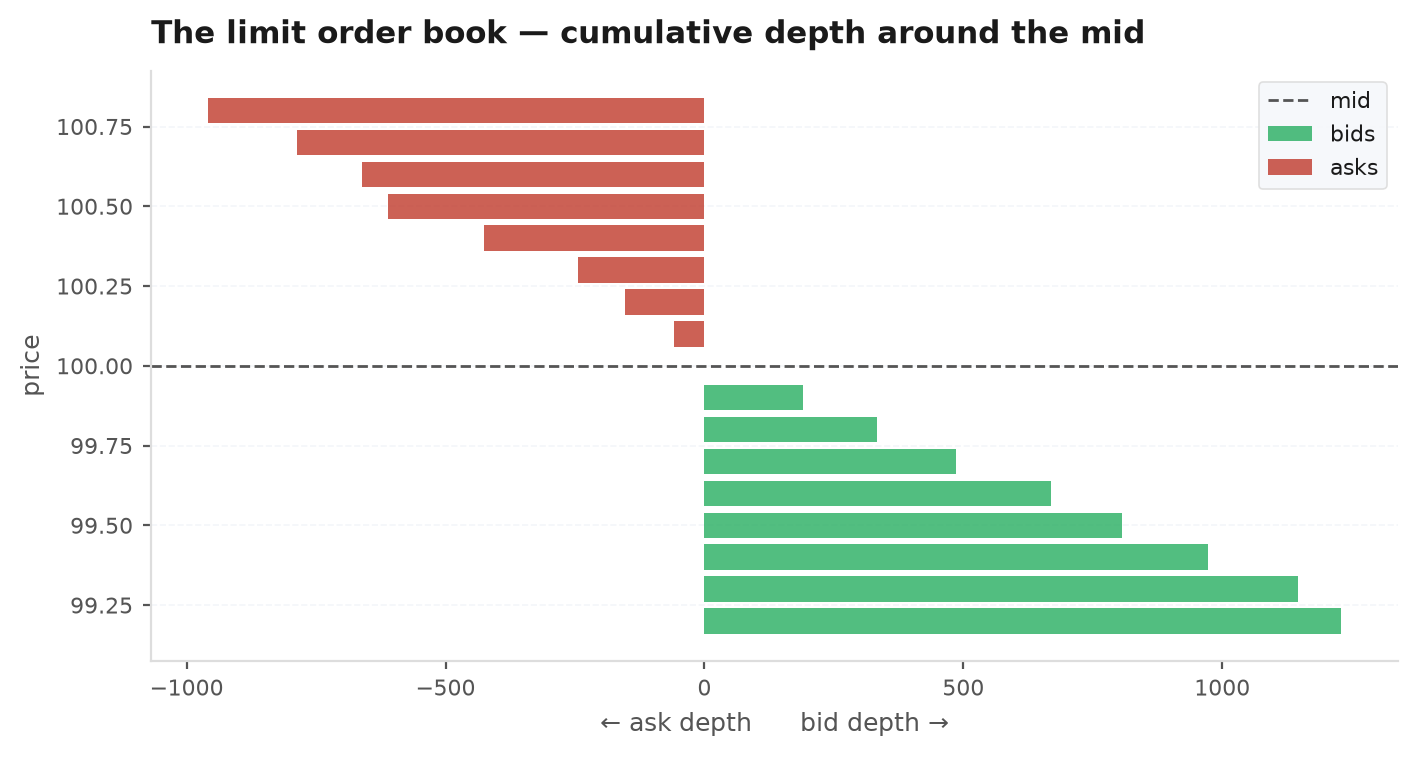
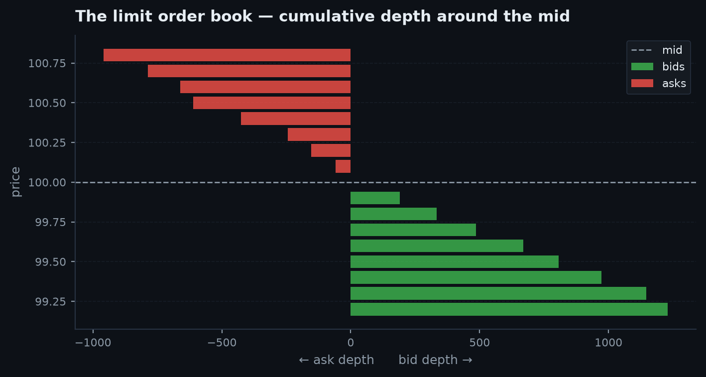
The quantities that decide whether a strategy survives — the spread, the impact per share, the toxicity of the order flow — live inside the limit order book, and most researchers never see a book. All you have is OHLCV bars. Remarkably, the bars remember: the bounce between bid and ask leaves a statistical fingerprint in the autocovariance of price changes, the spread leaves one in the daily ranges, and impact leaves one in the relation between returns and volume. This chapter is the toolkit for reading those fingerprints — ek.microstructure — and turning them into cost models, features, and regime filters.

✦Intuition — measuring the invisible

Imagine inferring the width of a doorway you cannot see by watching people stumble through it. Trades alternate between hitting the bid and lifting the ask, so the printed price hops back and forth across an invisible gap even when the true value never moves. That hop has a signature: an up-hop is more likely followed by a down-hop, so consecutive price changes are negatively correlated — and the strength of that negative correlation tells you how wide the gap is. Every estimator in this chapter is a version of this trick: find the statistical shadow that an unobservable microstructure quantity casts on observable bars, and invert it.

A limit order book drawn as horizontal bars: green bid depth stacked below the mid price, red ask depth above, with the bid-ask spread marked at the inside — What we are estimating: the book from the microstructure chapter. Bar data never shows you this ladder — but the spread and the depth leave recoverable traces in close-to-close changes, high-low ranges, and volume.

Roll’s model: the spread from closes alone#

Roll (1984) starts from the simplest possible model. The observed trade price is the true mid plus half a spread on one side or the other:

p_{t} = m_{t} + q_{t} \frac{s}{2}, q_{t} \in {+ 1, - 1} i.i.d., m_{t} a random walk

where $q_{t}$ is the trade direction (buy at the ask, sell at the bid) and $s$ the effective spread. Nothing else — no drift, no information. Yet this is enough to identify $s$ from closes.

✦Derivation — bid-ask bounce ⇒ negative autocovariance ⇒ s = 2√(−cov)

Difference the price: $Δ p_{t} = Δ m_{t} + \frac{s}{2} (q_{t} - q_{t - 1})$ . Now compute the first-order autocovariance. The mid is a random walk, so its increments contribute nothing across periods; only the bounce term survives:

Cov (Δ p_{t}, Δ p_{t - 1}) = \frac{s ^{2}}{4} E [(q_{t} - q_{t - 1}) (q_{t - 1} - q_{t - 2})] = - \frac{s ^{2}}{4}

since $E [q_{t} q_{t^{'}}] = 0$ for $t \neq = t^{'}$ and $E [q_{t - 1}^{2}] = 1$ . The bounce manufactures negative autocorrelation: a print at the ask tends to be followed by a print at the bid, so up-moves reverse. Invert:

s = 2 - Cov (Δ p_{t}, Δ p_{t - 1})

The catch: if genuine momentum makes the sample covariance positive, the square root is undefined — ek.microstructure.roll_spread returns nan rather than a fabricated number. That failure mode is informative: it means bounce is not the dominant effect at your sampling frequency.

Corwin-Schultz: the spread from highs and lows#

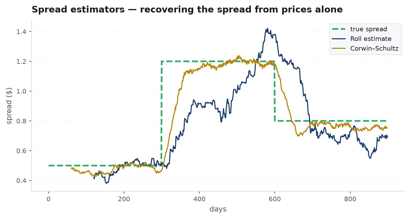
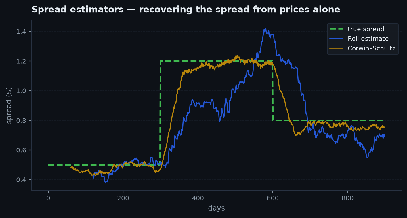
A second, independent read comes from the daily range. The insight: highs are almost always trades at the ask, lows are trades at the bid— so every observed high-low range contains the true mid’s range plus one full spread. Variance of the true range scales with time (two-day range variance is twice one-day), but the spread contribution does not: it is the same constant in a one-day range as in a two-day range. Comparing the sum of two single-day squared log-ranges with the squared two-day log-range therefore isolates the spread — the time-scaling part cancels differently from the constant part. With $β$ the sum of the two squared single-day log-ranges and $γ$ the squared two-day log-range, the closed form is

α = \frac{2 β - β}{3 - 2 2} - \frac{γ}{3 - 2 2}, s = \frac{2 ( e ^{α} - 1 )}{1 + e ^{α}}

corwin_schultz implements this per overlapping two-day window and clips at zero — noisy days can push the raw estimate negative, and a negative spread is a statement about sampling error, not markets. The practical appeal over Roll: it produces a time series of spread estimates from just highs and lows, so it can track widening liquidity day by day rather than delivering one number per sample.

→Both estimators are frequency-specific

Roll and Corwin-Schultz measure the spread at the frequency of the bars you feed them. Daily bars estimate the cost relevant to daily-horizon trading; intraday bars estimate a tighter effective spread. Neither estimator can see costs finer than its sampling grid — and both degrade when true-value moves within a bar dwarf the spread, which is why they are most reliable exactly where you need them most: quiet, small, illiquid names whose books you cannot see.

Roll and Corwin-Schultz spread estimates plotted through time against a true spread line, both tracking its level and widening during a stress episode — Two independent estimators, one truth. Roll (from close autocovariance) and Corwin-Schultz (from high-low ranges) both track the effective spread and both widen in stress — agreement between them is the sanity check that either is working.

Amihud illiquidity and Kyle’s lambda#

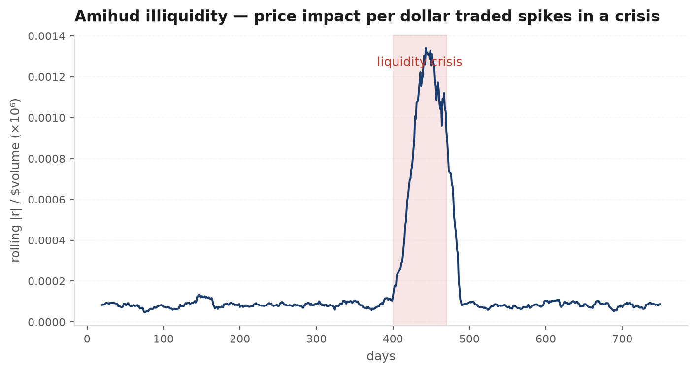
The spread prices smalltrades. For size, you want price impact per unit of volume. Amihud’s measure is the bluntest and most durable:

ILLIQ_{t} = \frac{∣ r _{t} ∣}{dollar volume _{t}}

— how much return one dollar of trading moves. Illiquid instruments move a lot on little volume. amihud reports a rolling mean scaled by $1 0^{6}$ (return per million dollars traded); it is a workhorse cross-sectional liquidity factor precisely because it needs nothing but bars.

Kyle’s $λ$ sharpens this into a regression with a sign. In Kyle’s model the market maker moves price linearly in net signed order flow: $Δ p_{t} = λ (q_{t} V_{t}) + ε_{t}$ . Bars do not record who initiated each trade, so the sign is estimated with the tick rule: an uptick is a buy, a downtick a sell, no change inherits the previous sign. kyle_lambda runs the rolling OLS of price change on tick-signed volume; the slope is dollars of impact per unit of net flow — the empirical cousin of the $η$ you fed into Almgren-Chriss.

Rolling Amihud illiquidity for a liquid and an illiquid instrument through time, the illiquid series an order of magnitude higher and spiking during market stress — Amihud illiquidity through time. The illiquid instrument sits an order of magnitude above the liquid one, and both spike together in stress — liquidity is a regime variable, and it vanishes exactly when everyone needs it.

VPIN and flow toxicity#

The most dangerous counterparty is an informed one. VPIN(volume-synchronised probability of informed trading) estimates how one-sided recent flow has been. Volume is cut into equal-size buckets (volume time, not clock time — activity speeds the clock up), each bucket’s volume is split into buy and sell pressure by bulk volume classification — assign a fraction $Φ (Δ p / σ_{Δ p})$ of the bucket to buys, the rest to sells, rather than signing each trade — and toxicity is the average absolute imbalance:

VPIN = \frac{1}{n} b = 1 \sum n \frac{∣ V _{b}^{buy} - V _{b}^{sell} ∣}{V _{b}}

High VPIN means flow is persistently one-sided — someone knows something, and liquidity providers, facing adverse selection, widen or withdraw. VPIN rose sharply in the hours before the 2010 flash crash; whatever its forecasting merits, it is a defensible statevariable for “how hostile is this tape right now.”

→VPIN is contested — use it as a thermometer, not an oracle

The academic fight over VPIN (did it predictthe flash crash, or merely rise with volatility?) is real: much of VPIN’s variation is explained by volatility itself, and its bucketing choices matter more than the theory suggests. That fight matters if you claim VPIN forecasts crashes; it matters much less for the defensive use here — a market maker or mean-reverter who stands down when bulk-classified imbalance is extreme is avoiding adverse selection whether the mechanism is information or volatility. Read it as a thermometer for hostile tape, and let the gauntlet judge any bolder claim.

From estimators to strategy inputs#

These are not just diagnostics — they are causal, bar-computable series, which makes them legal features and filters:

Estimator	Measures	Typical use
roll_spread	Effective spread (level)	Cost model input; universe screening
corwin_schultz	Spread (time series)	Regime filter: stand down when spreads blow out
amihud	Impact per dollar traded	Position-size cap; cross-sectional liquidity factor
kyle_lambda	Impact per unit signed flow	Calibrating execution models; capacity estimates
vpin	Flow toxicity	Risk-off switch for market-making / mean-reversion

The regime-filter use deserves emphasis: a mean-reversion edge that works at a 5 bps spread dies at 30 bps, so gating entries on corwin_schultz staying below a threshold is a structural filter, not curve fitting — the same logic as the regime detection chapter, with liquidity as the regime.

liquidity_gate.py

import edgekit as ek

# a causal liquidity regime filter: lag everything one bar, then gate
spread = ek.microstructure.corwin_schultz(bars["high"], bars["low"]).rolling(5).mean()
tox    = ek.microstructure.vpin(bars["close"], bars["volume"])

ok = (spread.shift(1) < 0.0015) & (tox.shift(1) < tox.shift(1).rolling(250).quantile(0.90))
signal = raw_signal.where(ok, 0.0)      # stand down when the tape is wide or toxic

Worked scenario — the spread from bars alone#

✦Scenario: a liquid ETF vs a small-cap, from daily closes

Two instruments, one year of daily bars each. The liquid ETF trades near $50 and its close-to-close changes show first-lag autocovariance $Cov (Δ p_{t}, Δ p_{t - 1}) = - 1.0 \times 1 0^{- 4} $^{2}$ . Roll:

s = 2 1.0 \times 1 0^{- 4} = $0.02 \Rightarrow 0.02/50 = 4 bps

The small-cap trades near $10 with autocovariance $- 6.25 \times 1 0^{- 4}$ : $s = 2 6.25 \times 1 0^{- 4} = $0.05$ — 50 bps, more than ten times the ETF’s relative spread. Now the sanity check that pays for the whole chapter: your backtest on the small-cap charged spread_rt=0.0012 (12 bps round trip) in its cost model. The bars themselves say a single crossing costs ~50 bps. The backtest is under-charging by roughly 8x, and the strategy’s 30 bps-per-trade edge is fiction. Estimate first, then set the cost model — never the other way around.

estimators.py

import edgekit as ek

# --- spread: two independent estimates ---
s_roll = ek.microstructure.roll_spread(bars["close"])          # scalar, $ per share
s_cs   = ek.microstructure.corwin_schultz(bars["high"], bars["low"])  # Series, relative
print(f"Roll: {s_roll/bars['close'].mean()*1e4:.0f} bps | CS median: {s_cs.median()*1e4:.0f} bps")

# --- impact: Amihud and Kyle's lambda (tick-rule signing inside) ---
illiq = ek.microstructure.amihud(bars["close"], bars["volume"], window=21)
lam   = ek.microstructure.kyle_lambda(bars["close"], bars["volume"], window=63)

# --- toxicity: VPIN in volume time ---
tox = ek.microstructure.vpin(bars["close"], bars["volume"], n_buckets=50, window=50)

# --- signing raw flow, if you need it directly ---
signs = ek.microstructure.tick_rule(bars["close"])             # +1 / -1 per bar

!Estimators are estimates

Every number above carries sampling error and model error. Roll assumes i.i.d. trade direction (momentum breaks it), Corwin-Schultz assumes highs and lows are quote-driven (overnight gaps break it), the tick rule misclassifies a material fraction of prints. Use them in pairs — when Roll and Corwin-Schultz agree, believe the level; when they diverge, believe neither and go find better data. And never let an estimator that reads price into a feature without lagging it — they are built from the same bars your strategy trades on.

Next: you can now measure your costs and your market. The next problem is allocating capital across several strategies when you do not yet know which is best — and never fully will. Bandits & online allocation.