Optimal execution

Execution & TCA established that trading costs money and that the cost grows with size. This chapter asks the next question: given that you must trade a large order, how should you spread it over time? Trade fast and you pay impact; trade slow and the price can run away from you. Almgren and Chriss turned that dilemma into a solvable optimisation — minimise expected cost plus a risk-aversion penalty on its variance — and the answer is a family of trajectories with TWAP at one end, immediacy at the other, and an efficient frontier of execution in between.

✦Intuition — the dealer’s dilemma

You hold a position you no longer want — say a million shares to sell. Dump it in one print and you crush the bid: the market charges you dearly for demanding all its liquidity at once. Drip it out over a week and each slice is nearly free — but for five days you are exposed to every headline, and the price may be 3% lower before you finish. Impact is the cost of certainty; timing risk is the cost of patience. Neither is avoidable, and the exchange rate between them depends on how much you fear an uncertain outcome. That fear has a name — risk aversion — and once you write it down as a number, the best schedule stops being a matter of taste and becomes a calculus problem with a closed-form answer.

Temporary vs permanent impact#

From microstructure: your order moves the price in two ways. Temporary impact is the concession for immediacy — you walk the book, depth refills, the price snaps back. It depends on the rate you trade at: in the Almgren-Chriss model, selling at speed $v$ costs an extra $η v$ per share. Permanent impact is the information your flow reveals — the mid shifts and stays shifted. It depends on total quantity, not speed, which is why (in the linear model) you cannot schedule your way out of it: only the temporary part and the timing risk are up for optimisation.

Market impact plotted against order size as a fraction of daily volume, a concave square-root curve rising steeply for small sizes then flattening — Impact vs participation, from the execution chapter. The concave shape is why slicing helps: many small slices ride the cheap, steep-discount part of the curve instead of paying the full-size price at once.

The square-root law#

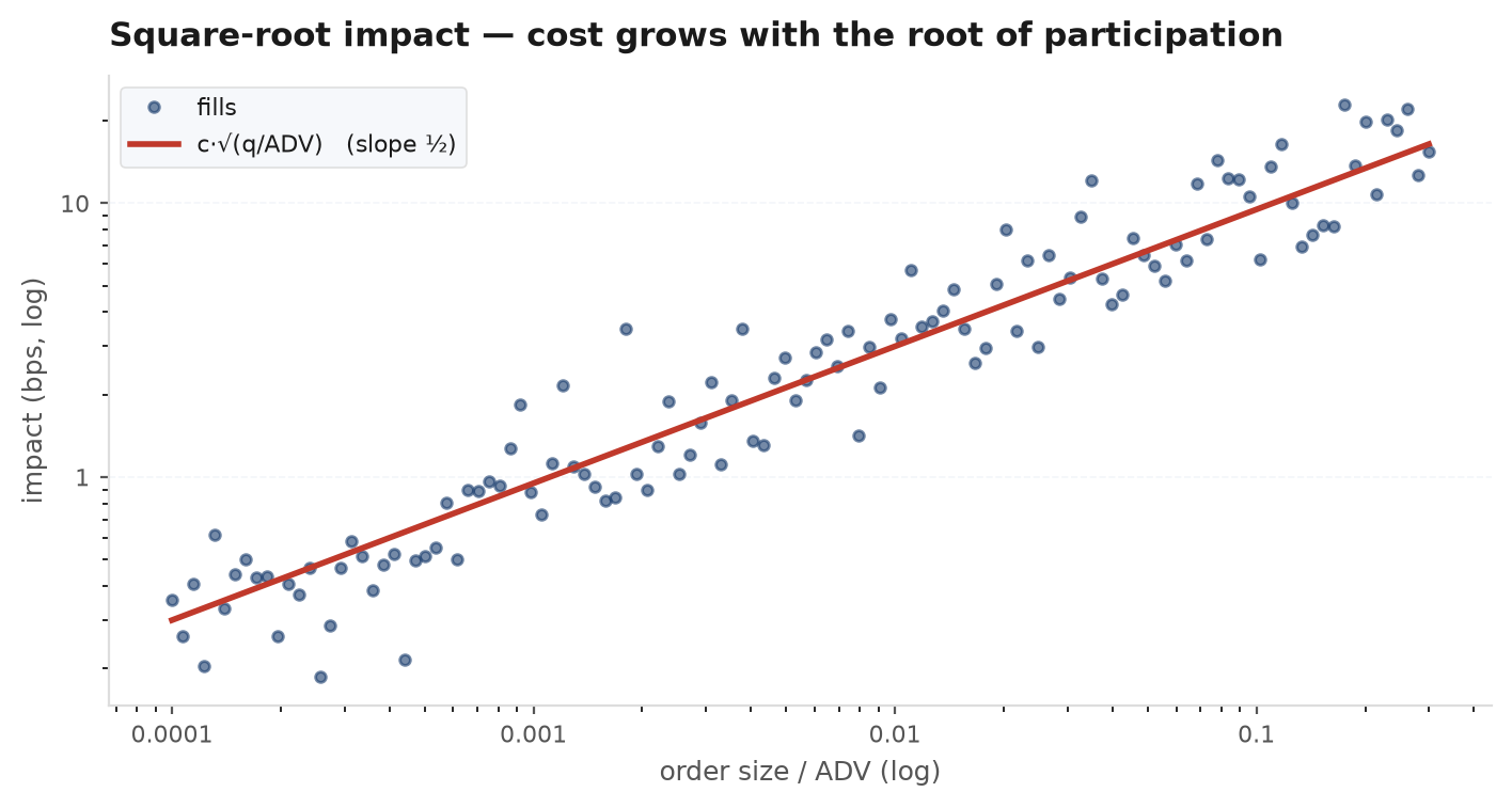
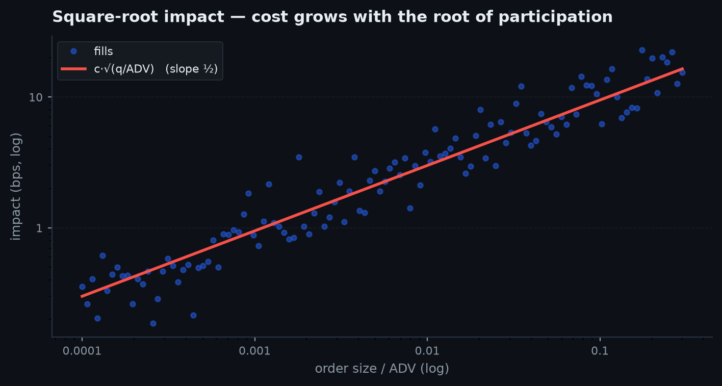
Before optimising, calibrate. The most robust empirical fact about impact — measured across equities, futures, FX, and crypto, across decades and venues — is that the total cost of executing a quantity $Q$ against average daily volume $V$ scales as

impact \approx c σ_{daily} \frac{Q}{V}, c \approx 0.5 - 1.0

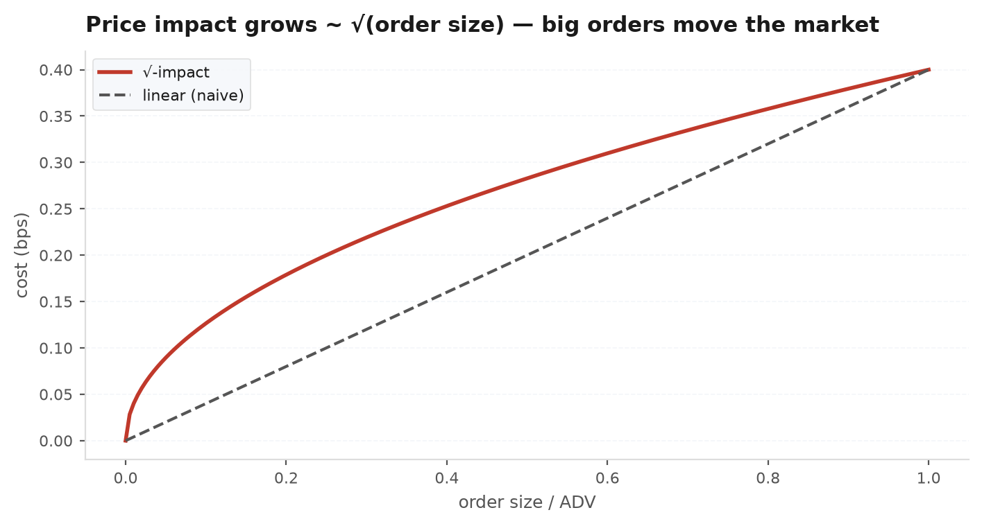
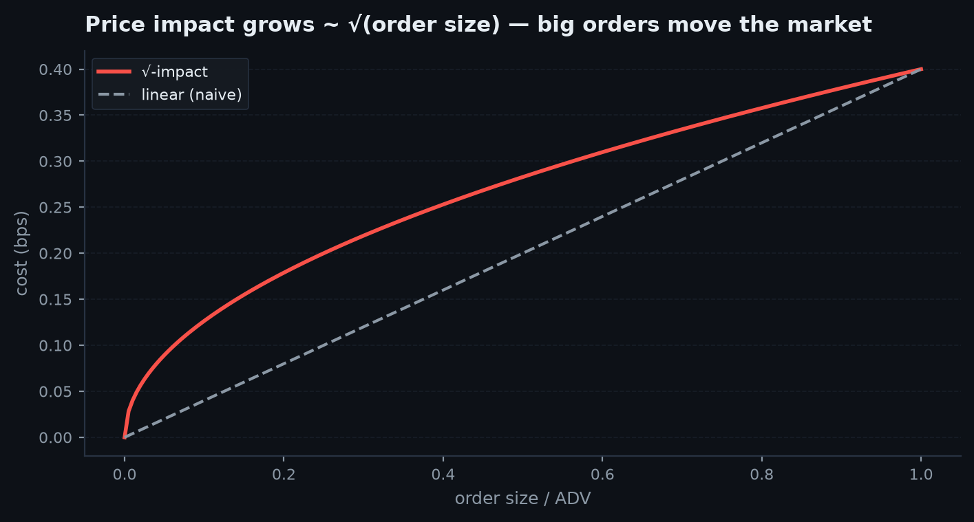
with $σ_{daily}$ the daily volatility. The remarkable part is the universality: the same exponent, close to $1/2$ , shows up in markets that share nothing but the auction mechanism. It is not what naive linear reasoning predicts — doubling size less than doubles cost — and that concavity is precisely what makes scheduling worthwhile. The law prices the whole order; the Almgren-Chriss machinery below decides how to spend that budget through time.

Empirical impact measurements against participation rate on log-log axes, collapsing onto a line of slope one half — The square-root law. Measured impact against participation Q/V follows a slope-1/2 power law across instruments — one of the few empirical regularities in trading robust enough to build a cost model on.

The Almgren-Chriss problem#

Hold $x_{0}$ shares to liquidate over horizon $T$ , split into $n$ intervals. A trajectory $x_{0}, x_{1}, \dots, x_{n} = 0$ is a plan for how much remains at each step. Every trajectory has an expected cost $E [C]$ (impact — higher when you trade fast) and a variance $Var [C]$ (timing risk — higher when inventory lingers). Almgren-Chriss picks the trajectory minimising

x_{1}, \dots, x_{n - 1} min E [C] + λ Var [C]

where $λ \geq 0$ is your risk aversion — the same mean-variance logic as portfolio construction, applied to a single order.

✦Derivation — from mean-variance to the sinh trajectory

With linear temporary impact $η$ , trading $v_{j} = x_{j - 1} - x_{j}$ shares in interval $j$ of length $τ$ costs $η v_{j}^{2} / τ$ ; holding $x_{j}$ shares through an interval contributes $σ^{2} τ x_{j}^{2}$ to the variance. The objective is

j \sum \frac{η v _{j}^{2}}{τ} + λ σ^{2} τ j \sum x_{j}^{2} .

In the continuous limit this is a calculus-of-variations problem; the Euler-Lagrange equation is $x ¨ = κ^{2} x$ with

κ = \frac{λ σ ^{2}}{η}

— impatience rises with risk aversion and volatility, falls with impact cost. With boundary conditions $x (0) = x_{0}$ , $x (T) = 0$ , the solution is the hyperbolic sine trajectory:

x (t) = x_{0} \frac{sinh ( κ ( T - t ) )}{sinh ( κ T )} .

Read the limits. As $λ \to 0$ (indifferent to risk), $κ \to 0$ and $x (t) \to x_{0} (1 - t / T)$ — a straight line, which is exactly TWAP: pure impact-minimisation ignores timing risk. As $λ \to \infty$ , $κ T$ blows up and the trajectory collapses toward immediate liquidation — dump everything, pay the impact, sleep at night. Every real schedule lives between those poles, and $κ T$ is the single dimensionless number that says where.

The efficient frontier of execution#

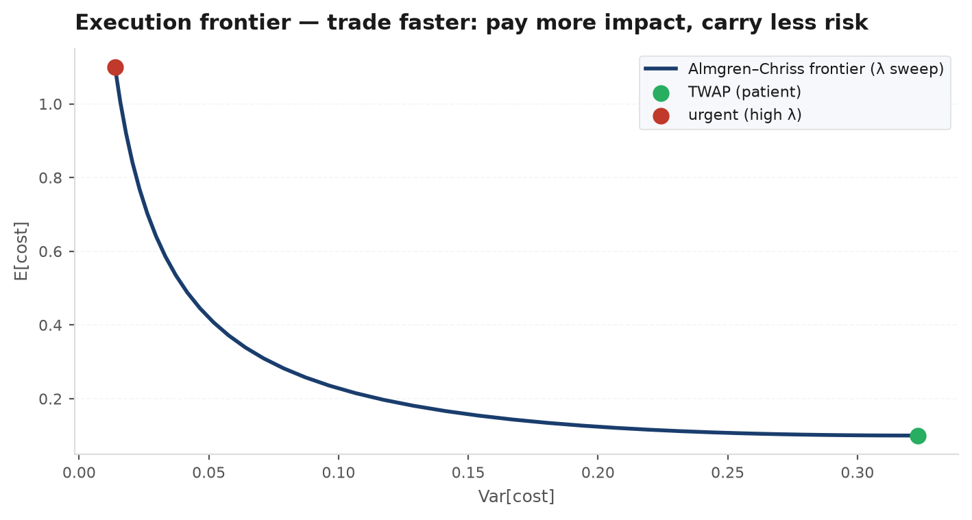
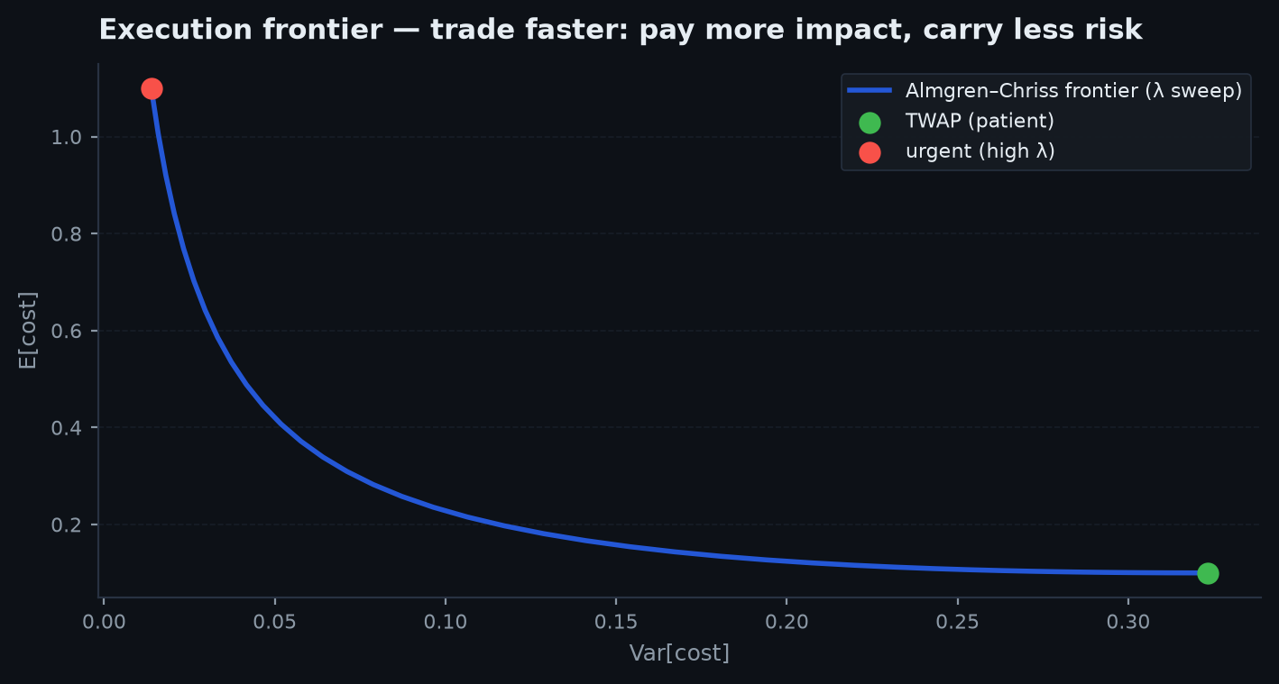
Sweep $λ$ from zero upward and each optimal trajectory traces one point in the (variance, expected cost) plane. The result is an efficient frontier: no schedule exists below it, and every schedule above it is dominated — same risk, more cost. TWAP sits at the frontier’s minimum-cost, maximum-variance end; instant liquidation at the opposite corner. VWAP is a practical refinement of the TWAP end: it spends the same schedule in volume time rather than clock time, concentrating slices when the market is busy so instantaneous participation stays constant. Choosing an execution algo without choosing $λ$ is choosing a frontier point at random.

The Almgren-Chriss efficient frontier: expected execution cost against cost variance, a convex curve with TWAP at the low-cost high-variance end and rapid liquidation at the high-cost low-variance end — The efficient frontier of execution. Each point is the optimal trajectory for one risk aversion. TWAP (lower right) minimises expected impact but leaves inventory exposed longest; front-loaded schedules (upper left) buy certainty with impact.

Implementation shortfall, decomposed#

Perold’s implementation shortfall is the scorecard: the gap between the paper portfolio (filled at the decision price, free) and the real one. It decomposes along the timeline of the order:

IS = delay cost (P_{arrival} - P_{decision}) + execution cost (P ˉ_{fill} - P_{arrival}) + opportunity cost

(signs flip for a sell). Delay is what the price did between deciding and reaching the market — a process problem. Execution is spread plus impact against arrival — the part the AC schedule manages. Opportunity is the drift on anything you never filled. Decomposing tells you which part of your pipeline leaks; a single blended number does not.

→Which piece belongs to whom

The decomposition assigns blame. Persistent delay cost means your signal-to-order pipeline is slow — an engineering fix, not a trading one. Execution cost above the square-root-law estimate means the schedule or the venue is wrong. Chronic opportunity cost means you are systematically too passive on the orders that matter most — which, since your orders correlate with your signal, is adverse selection against yourself. Averaging the three into one number hides all three diagnoses; this is why implementation_shortfall returns the split, not just the total.

A useful discipline: before any large order, write down the three numbers you expect — square-root-law impact for the size, the AC split of that budget for your $λ$ , and zero delay. After the fill, the realised decomposition against those expectations is the fastest error signal your execution process gets, and feeding it back is what keeps the cost model honest for the backtest-to-live reconciliation later.

Worked scenario — selling 5% of ADV#

✦Scenario: 1m shares of a $40 stock, one day to do it

You must sell $Q = 1, 000, 000$ shares of a $40 stock with ADV $V = 20$ m shares and daily volatility $σ = 2%$ — a 5%-of-ADV order. First, the budget from the square-root law with $c = 1$ :

impact \approx 1.0 \times 0.02 \times 0.05 \approx 0.0045 \approx 45 bps

— about 18 cents a share, $$179, 000$ on the $40m notional. That is the full-order price; the schedule decides the impact/risk split. Timing risk of holding the position all day is $σ \times $40 m = $800, 000$ of one-day standard deviation — more than four times the impact budget, which is why pure TWAP feels reckless here. With a moderate risk aversion giving $κ T \approx 2$ , the AC schedule sells roughly half the order in the first third of the day: expected cost rises perhaps 20% above the TWAP minimum, but the standard deviation of the outcome falls by nearly half. On the frontier plot, that is the region where the curve is steep — cheap variance reduction. Whether you take it is exactly what $λ$ encodes.

ac_schedule.py

import numpy as np
import edgekit as ek

# --- budget: square-root law, selling 5% of ADV ---
frac = ek.execution.sqrt_impact(q=1_000_000, adv=20_000_000, sigma_daily=0.02, c=1.0)
print(f"sqrt-law impact ~ {frac*1e4:.0f} bps")            # ~45 bps

# --- Almgren-Chriss over one day, 26 x 15-minute slices ---
ac = ek.execution.almgren_chriss(
    x0=1_000_000, t=1.0, n=26,
    sigma=0.80,          # $/share/day  (2% of $40)
    eta=2.5e-6,          # temporary-impact coefficient
    lam=2e-6,            # risk aversion
)
print(f"kappa={ac.kappa:.2f}  E[cost]=${ac.expected_cost:,.0f}  sd=${np.sqrt(ac.cost_variance):,.0f}")
slices = -np.diff(ac.trajectory)                           # shares per interval (front-loaded)

# --- the two benchmark limits ---
twap = ek.execution.twap_schedule(qty=1_000_000, n=26)     # equal slices
vwap = ek.execution.vwap_schedule(qty=1_000_000, volume_profile=intraday_volume)  # U-shaped

shortfall.py

# score the realised execution against the decision price
res = ek.execution.implementation_shortfall(
    decision_price=40.00,
    fill_prices=fills["price"],   # per-slice average fills
    fill_qtys=fills["qty"],
    side=-1,                      # selling
    arrival_price=39.96,          # mid when the order reached the market
)
print(f"total {res['total_bps']:.1f} bps = delay {res['delay_bps']:.1f} + execution {res['execution_bps']:.1f}")
print(f"avg fill {res['avg_fill']:.4f}")

What the model assumes#

Almgren-Chriss assumes	Reality	Consequence
Linear temporary impact η·v	Impact is concave (square-root) in rate	AC over-penalises large slices; real optima front-load less
Known, constant σ and η	Both spike exactly when you must trade	Recalibrate intraday; treat κ as a dial, not a constant
Arithmetic random-walk price	Drift, momentum, and news mid-order	Adverse drift argues for faster schedules than λ alone implies
No one reacts to your flow	Predators detect predictable schedules	Randomise slice timing; avoid clockwork TWAP footprints

!The schedule is optimal only inside its model

The sinh trajectory is exact under linear impact and Gaussian noise — and the world is neither. Treat AC the way you treat mean-variance optimisation: not as truth but as a disciplined way to turn beliefs (sigma, eta, lam) into a defensible schedule, stress-tested like any other model. The empirical square-root law is the reality check the linear model must be calibrated against.

Everything above assumed you know the spread, the impact coefficient, the toxicity of the flow around you. From bar data alone, those quantities are invisible — but they can be estimated.

Next: Microstructure estimators— Roll, Corwin-Schultz, Amihud, Kyle’s lambda, and VPIN: measuring spread, illiquidity, and flow toxicity from nothing but OHLCV.