Bandits & online allocation

You run a book of three strategies. One of them is better than the others — but you do not know which, and every day of data is too noisy to settle it. Give capital to the wrong one and you bleed opportunity; split evenly forever and you never harvest what you learn. This is the multi-armed bandit problem, and it has a beautiful theory: optimism-under-uncertainty (UCB), posterior sampling (Thompson), and regret bounds that say how little you must lose while learning. This chapter builds that theory, then confronts it with the fact that makes markets special — the arms do not sit still.

✦Intuition — the explore/exploit dilemma

A casino has three slot machines with different, unknown payout rates. Every pull spent on a worse machine is money lost to learning; every pull spent on the current favourite risks never discovering it was not the best. Pure exploitation locks in early noise — the machine that got lucky in its first ten pulls keeps all your coins. Pure exploration pays full tuition forever. The entire field of bandit algorithms is the mathematics of the middle path: allocate moreto what looks good, but never let an arm’s trial count get so low that you could be wrong about it cheaply. Swap “machines” for “strategies” and “pulls” for “capital-days” and you have the daily job of running a book.

The bandit problem and regret#

Formally: $K$ arms, arm $i$ paying i.i.d. rewards with unknown mean $μ_{i}$ ; each round you choose an arm (or a weighting over arms) and observe the outcome. The scorecard is regret — what the best arm in hindsight earned, minus what you earned:

R_{T} = T μ^{*} - t = 1 \sum T μ_{a_{t}}, μ^{*} = i max μ_{i}

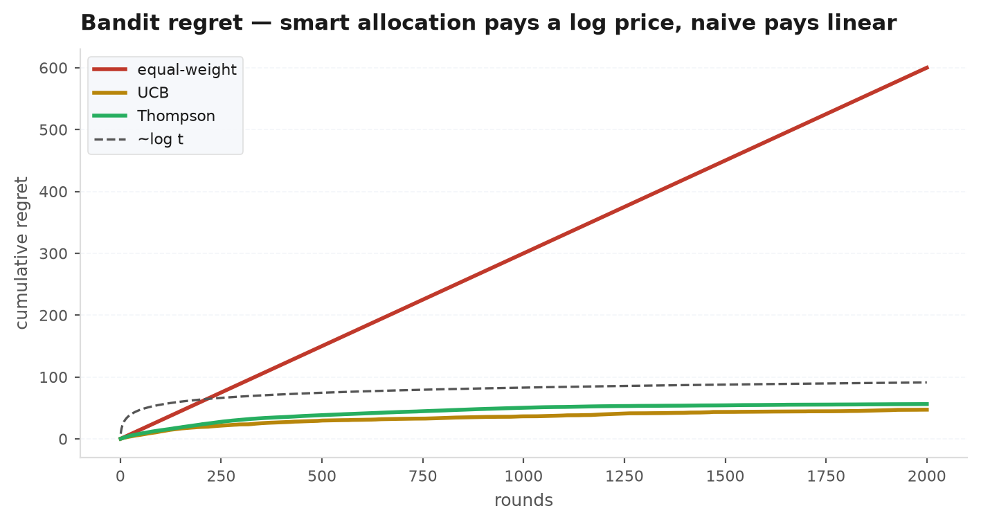
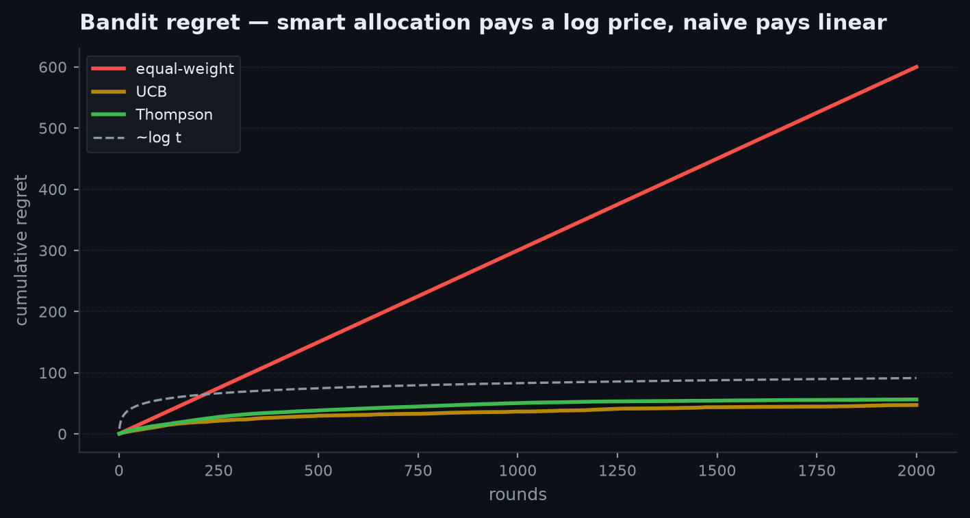
A strategy that learns has regret growing sublinearly — the per-round cost of not knowing shrinks to zero. The landmark result (Lai-Robbins): no algorithm can beat $O (ln T)$ regret on hard instances, and good algorithms achieve it. Logarithmic regret means the tuition for learning which strategy is best is a bounded fractionof your P&L that vanishes as time passes — a remarkably cheap education, if the world holds still.

UCB: optimism under uncertainty#

Upper Confidence Bound picks, each round, the arm with the highest optimistic estimate: sample mean plus a bonus that grows with uncertainty:

a_{t} = ar g i max μ^_{i} + \frac{2 ln t}{n _{i}}

where $n_{i}$ is how often arm $i$ has been tried. Arms you have barely sampled carry big bonuses and get tried; arms sampled often must earn their keep on the mean alone.

✦Derivation — Hoeffding’s inequality ⇒ the optimism bonus

Hoeffding: for $n$ i.i.d. bounded rewards, the sample mean concentrates as

Pr (μ_{i} > μ^_{i} + ε) \leq e^{- 2 n_{i} ε^{2}} .

Demand that the true mean exceeds our optimistic bound with probability at most $δ = t^{- 4}$ (shrinking fast enough that mistakes are summable over all rounds and arms). Solve $e^{- 2 n_{i} ε^{2}} = t^{- 4}$ for $ε$ :

ε = \frac{2 ln t}{n _{i}}

— exactly the UCB bonus. The logic: with high probability, everyarm’s true mean lies below its optimistic index; so if you keep pulling the highest index, a suboptimal arm can only be pulled while its bonus still covers its gap $Δ_{i} = μ^{*} - μ_{i}$ , which happens at most about $8 ln T / Δ_{i}^{2}$ times. Total regret: $\sum_{i} Δ_{i} \cdot O (ln T / Δ_{i}^{2}) = O (ln T)$ . Optimism is not a heuristic — it is a concentration inequality worn as a decision rule.

Thompson sampling: allocate by belief#

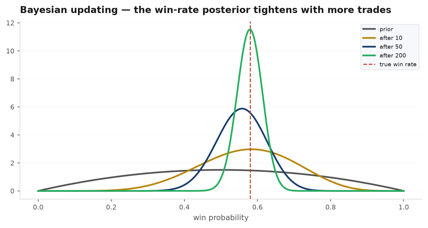
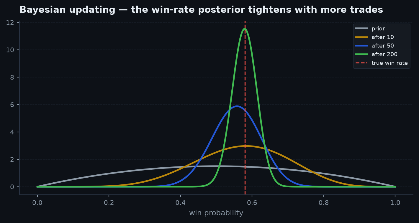
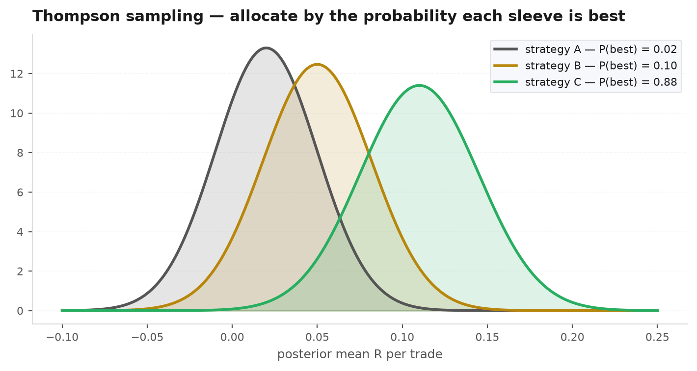
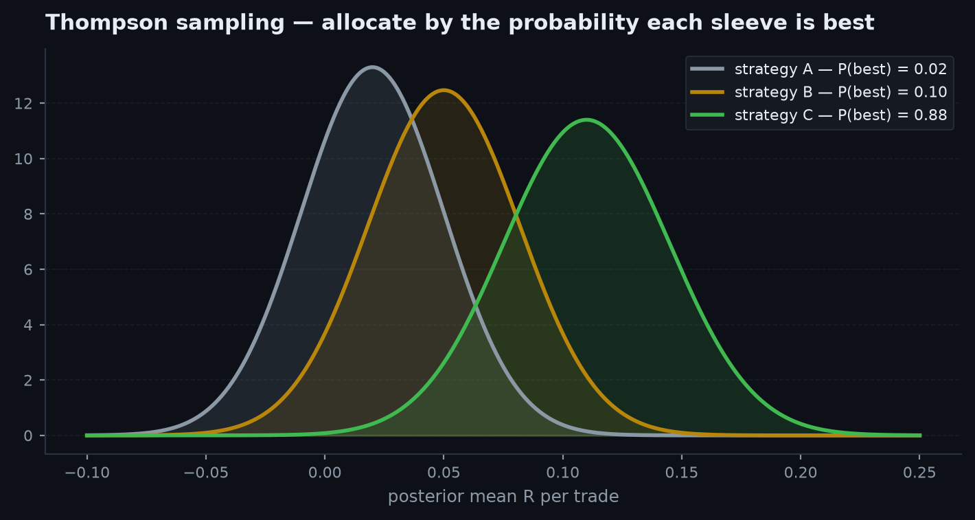
Thompson sampling is the Bayesian sibling, and older than all of it (1933). Maintain a posterior over each arm’s mean; each round, draw one sample from each posterior and play the arm whose draw is highest. Arms are chosen with exactly the probability that they are the best, given everything seen so far — exploration emerges from posterior width, no bonus term needed. This is the Bayesian updatingmachinery doing allocation: wide posteriors (little data) produce occasional optimistic draws and get explored; as evidence accumulates, posteriors sharpen and the best arm’s draws dominate. For a book of strategies the translation is direct: capital share = posterior probability of being the best strategy, which is what ek.allocate.thompson computes from a returns frame.

✦Derivation — the posterior a returns column carries

For strategy returns, the natural conjugate model is Normal with (approximately) known variance: after $n_{i}$ observations with sample mean $μ^_{i}$ and volatility $σ_{i}$ , a flat prior gives the posterior over the true mean

μ_{i} data \sim N (μ^_{i}, \frac{σ _{i}^{2}}{n _{i}})

— the same standard error that runs through the whole statistics course, now read as a belief. Thompson allocation draws $μ ~_{i} \sim N (μ^_{i}, σ_{i}^{2} / n_{i})$ for each column, awards the round to the largest draw, and repeats a few thousand times; the win frequencies are the weights. Note what the formula implies: with equal track-record lengths, exploration is driven entirely by the ratio of mean gaps to standard errors — the bandit is automatically humble exactly when the t-statistics say it should be.

Beta posterior distributions sharpening as evidence accumulates over successive updates — From the Bayesian chapter: posteriors sharpen with evidence. Thompson sampling turns this straight into allocation — each strategy's capital share is the probability mass on 'this one is best'.

Three posterior distributions over strategy mean returns at an early and a late date, overlapping heavily at first and separating later as the best strategy's posterior pulls right — Three strategies' posteriors over mean daily R, early (heavy overlap — allocation near equal) and late (the best arm's posterior has pulled away — it now wins most draws and most capital). Thompson's allocation is just this picture, integrated.

Why markets are not stationary bandits#

Every guarantee above leans on one assumption: $μ_{i}$ is constant. Markets violate it structurally. Edges decay — crowding, regime change, the very act of trading them. A bandit algorithm that has “solved” the book keeps allocating to the historical winner long after its edge is gone; the theory calls these restless bandits, and their clean guarantees mostly evaporate. Two practical consequences:

Never let exploration die. Stationary algorithms sample losing arms at a rate $\to 0$ . Against drifting means you must keep a floor on every arm’s allocation, or you cannot detect a revival — or a death.
Discount old evidence. A return from three years ago says little about an edge today. ek.allocate.ewma_weightsis the pragmatic middle ground: exponentially-weighted mean over exponentially-weighted vol, half-life ~a quarter — a bandit that deliberately forgets. Monitor each sleeve’s decay explicitly with ek.metrics.edge_decay, which fits a trend to rolling expectancy and reports its t-statistic.

Worked scenario — three strategies, one secretly better#

✦Scenario: 0.02R, 0.02R, and a hidden 0.05R per day

Three strategies with daily R-multiples of standard deviation $\approx 1$ R. Two have true expectancy $0.02$ R/day, one has $0.05$ R/day — but with noise 20-50x the daily signal, a year of data gives each mean a standard error of $1/ 252 \approx 0.063$ R: twice the gap you are trying to detect. No t-test will settle this in a year. Run the allocators for 500 trading days:

Equal weight earns the average, $0.03$ R/day — regret grows linearly at $0.02$ R/day, ~10R over the run. The price of never learning.
Thompsonstarts near equal (posteriors overlap almost completely), and by day ~300 the good arm’s share drifts to ~60%; realised expectancy ~ $0.038$ R/day and the regret curve is visibly bending. It never hits 100% — with this signal-to-noise it shouldn’t, because the posterior genuinely is not sure.
UCB tracks a similar path, more mechanical: the laggards keep earning trial allocations whenever their confidence bonus (shrinking like $ln t / n_{i}$ ) covers the observed gap.

The honest summary: bandits do not find the winner fast — nothing can, at this noise level. They lose less while not knowing, and they concentrate exactly as fast as the evidence justifies. That is the entire, and sufficient, sales pitch.

Cumulative regret curves for equal-weight, UCB, and Thompson allocation: equal weight rising linearly, UCB and Thompson bending toward logarithmic growth — Regret over 500 days on the three-strategy book. Equal weight pays a constant per-day tuition (linear). UCB and Thompson bend — the hallmark of learning — approaching the log t shape the theory promises for stationary arms.

allocate.py

import edgekit as ek

# rets: DataFrame of daily R per strategy, columns = ["mom", "revert", "carry"]
w_ts  = ek.allocate.thompson(rets, n_draws=2000)    # P(each col is best) as weights
w_ucb = ek.allocate.ucb(rets, c=2.0)                # mean + c*se, floored at 0, normalised
w_ew  = ek.allocate.ewma_weights(rets, halflife=63) # forgetting allocator (non-stationary world)

# tuition paid so far: best-in-hindsight minus realised
reg = ek.allocate.regret(rets)                      # equal-weight benchmark
print(f"cumulative regret: {reg.iloc[-1]:.1f}R")

# is any sleeve dying? trend in rolling expectancy, with CI
decay = ek.metrics.edge_decay(rets["mom"], window=50)
print(f"decay slope t-stat: {decay.attrs['slope_t']:.2f}")   # deeply negative = retire it

Allocator	Assumes	Strength	Weakness
Equal weight	Nothing	Unbeatable when arms are truly indistinguishable	Pays linear regret when they are not
UCB	Stationary means, bounded noise	Distribution-free log-regret guarantee	Bonus mis-scaled for heavy-tailed R streams
Thompson	A posterior you believe	Allocates by belief; integrates priors naturally	Same stationarity blind spot, dressed in Bayes
EWMA weights	Recent past predicts near future	Tracks drifting and dying edges	No optimality guarantee; halflife is a judgment call

The bandit view also reframes a familiar object: a parameter sweep is a bandit where each configuration is an arm — and running the full sweep, picking the best, and betting it all is the maximal-exploitation corner solution whose regret properties are exactly why PBO and deflated Sharpe exist. Online allocation across configurations, with a floor and a forgetting factor, is the sequential version of the same multiple-testing discipline.

!A bandit is not a risk manager

Allocation weights answer “who gets the capital?” — not “how much risk in total?” Run the bandit on relative shares inside a book whose total risk is set by the sizing and risk framework, and let correlation between sleeves into the decision the way portfolio construction taught — three momentum strategies are not three independent arms, whatever the bandit thinks. And a strategy whose edge_decay slope has gone significantly negative should be retired by policy, not merely starved by posterior.

Thompson and UCB decide how to divide capital while you learn — a graded, continuous response to accumulating evidence. But there is a sharper, binary version of the same question that every live trader faces: is the strategy I am currently runningstill the one I backtested — or has it quietly died? A bandit starves a dying arm slowly, at the rate its posterior sours; a monitor’s job is to call it, with a controlled error rate, so that policy — not drift — retires the strategy.

Next: Monitoring a live strategy — sequential tests, CUSUM alarms, probabilistic Sharpe, and kill-switch design: deciding noise-or-death with data you collect one day at a time.