Probability & distributions

A return is a random variable — you cannot know tomorrow’s, only its distribution of possibilities. Trading is the business of taking bets whose average outcome is positive while surviving the tails. This chapter builds the vocabulary — expectation, variance, the Normal, and crucially why markets are not Normal — that the rest of the course reasons in.

Random variables & expected value#

A random variable $X$ is a quantity whose value is uncertain — a trade’s return, tomorrow’s move. Its expected value $E [X]$ is the probability-weighted average outcome: the long-run mean if you could replay the bet forever. For a discrete variable:

E [X] = i \sum x_{i} p (x_{i})

and for a continuous one, the integral against its density $f (x)$ :

E [X] = \int_{- \infty}^{\infty} x f (x) d x

Expectation is linear: $E [a X + bY] = a E [X] + b E [Y]$ , always, even when $X$ and $Y$ are dependent. This is the engine behind expectancy — a strategy’s edge is just the expected value of one trade, and the total is the sum of the parts. It is the single most important quantity in the whole course.

Proof: linearity of expectation#

Linearity is worth proving once because it holds unconditionally — no independence required — and that is exactly what makes expectancy add up trade by trade.

→Derivation — sum over the joint distribution

Let $p (x, y)$ be the joint probability of $X = x$ and $Y = y$ . By definition,

E [a X + bY] = x \sum y \sum (a x + b y) p (x, y)

Split the sum and pull the constants out:

= a x \sum x y \sum p (x, y) + b y \sum y x \sum p (x, y)

The inner sums are just the marginals — $\sum_{y} p (x, y) = p_{X} (x)$ and $\sum_{x} p (x, y) = p_{Y} (y)$ — so

= a x \sum x p_{X} (x) + b y \sum y p_{Y} (y) = a E [X] + b E [Y] . ■

Nothing above assumed $X$ and $Y$ were independent — the joint distribution carried all the dependence, and it dropped out.

✦Why it matters for trading

Linearity is why a strategy’s total expected profit is the sum of its trades’ expectancies even though the trades are correlated (same regime, overlapping positions). You can add up edges without untangling their dependence — but, as we will see, you cannot add up their variances that way.

Random variables, PDF and CDF#

Two functions fully describe a continuous random variable. The cumulative distribution function (CDF) gives the probability of landing at or below a level — it runs monotonically from 0 to 1:

F (x) = P (X \leq x), F (- \infty) = 0, F (+ \infty) = 1

The probability density function (PDF) is its derivative, $f (x) = F^{'} (x)$ , so probability is area under the density: $P (a < X \leq b) = \int_{a}^{b} f (x) d x = F (b) - F (a)$ . A single point has zero probability; only intervals carry mass. The CDF is the object behind quantiles and VaR (later on this page); the PDF is the bell curve you picture.

✦Scenario: the expected value of one ORB trade

Picture an opening-range breakout on US100 that risks 1R to make 2R. Historically it wins 40% of the time. Model one trade as a random variable

R

: it pays

+ 2

with probability 0.40 and

- 1

with probability 0.60. Its expected value is

E [R] = (0.40) (+ 2) + (0.60) (- 1) = 0.8 - 0.6 = + 0.2 R

. So on average each trade adds a fifth of a risk unit. But look at what you actually experience: no single trade ever returns

+ 0.2 R

— every outcome is either

+ 2 R

- 1 R

, and the more common one is a loss. The

+ 0.2 R

is the center of gravity you drift toward over hundreds of trades, not a forecast of the next one. That is why a losing streak can be perfectly consistent with a real positive expectancy.

→Expectation is not what you will get

E [X]

is the center of gravity of the distribution, not a prediction of any single draw. A coin flip paying +2 or −1 has

E [X] = 0.5

, but no individual flip ever returns 0.5. Edge is a statement about the average of many trades — the theme of The math of edge.

Variance & standard deviation#

Expectation tells you the center; variance tells you the spread. It is the expected squared distance from the mean:

Var (X) = σ^{2} = E [(X - μ)^{2}] = E [X^{2}] - μ^{2}

→Derivation — the computational identity

The far-right form $E [X^{2}] - μ^{2}$ is the one you actually compute with. Expand the square inside the expectation and use linearity, remembering $μ = E [X]$ is a constant:

Var (X) = E [(X - μ)^{2}] = E [X^{2} - 2 μ X + μ^{2}] = E [X^{2}] - 2 μ E [X] + μ^{2}

Since $E [X] = μ$ , the middle term is $- 2 μ^{2}$ and it collapses:

= E [X^{2}] - 2 μ^{2} + μ^{2} = E [X^{2}] - μ^{2} . ■

A useful corollary: because a variance can never be negative, $E [X^{2}] \geq (E [X])^{2}$ always — a special case of Jensen for the convex function $x^{2}$ .

Squaring makes it awkward to read (units of return-squared), so we usually quote the standard deviation $σ = Var (X)$ , which is back in the units of the return itself. In finance $σ$ is called volatility, and it is the denominator of the Sharpe ratio and the raw material of position sizing.

A key scaling fact: for independent returns, variance adds over time, so volatility grows with the square root of the horizon. Daily vol annualises as $σ_{ann} = σ_{daily} 252$ . That $N$ shows up again in the standard error and in the Sharpe annualisation — it is the same idea each time.

Covariance, correlation & diversification#

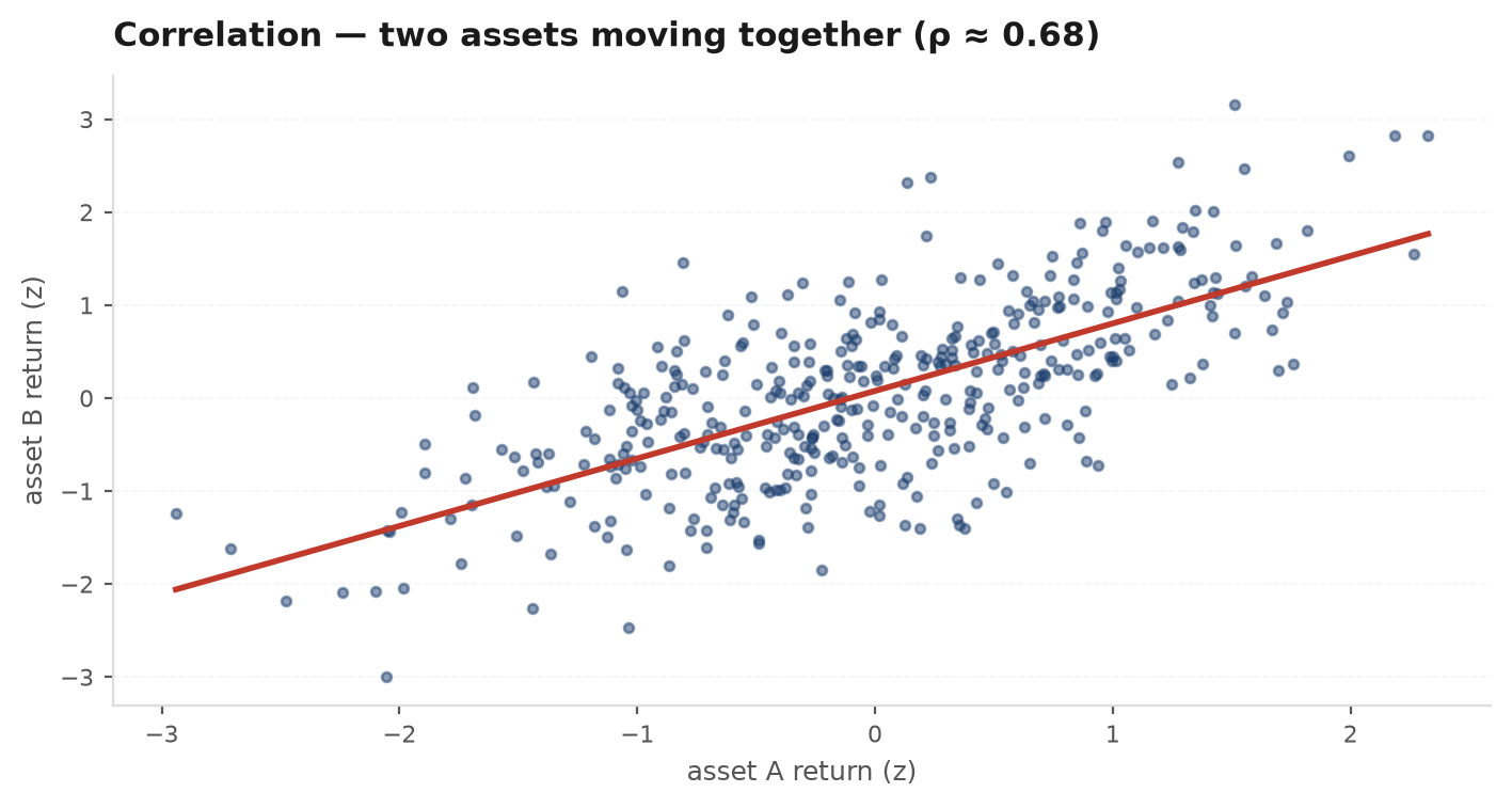
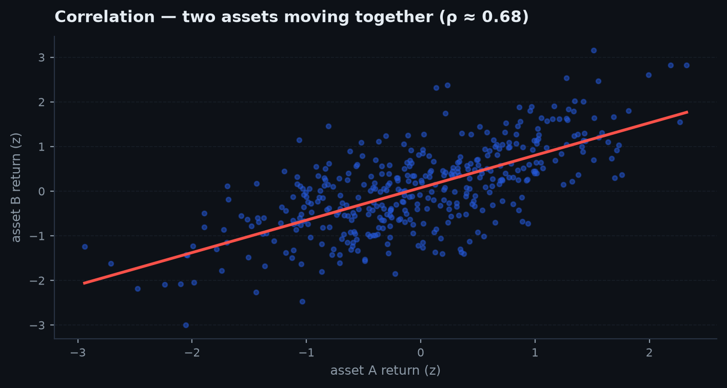
Variance describes one variable in isolation. Covariance measures how two move together — the expected product of their deviations from their means:

Cov (X, Y) = E [(X - μ_{X}) (Y - μ_{Y})] = E [X Y] - μ_{X} μ_{Y}

Positive covariance: when one is above its mean the other tends to be too. The second form comes from the same expand-and-cancel trick as the variance identity (indeed $Cov (X, X) = Var (X)$ ). Covariance is hard to read on its own because its units are the product of the two variables’ units, so we normalise it into the unitless correlation coefficient:

ρ_{X Y} = \frac{Cov ( X , Y )}{σ _{X} σ _{Y}} \in [- 1, 1]

Scatter of two assets' returns with a fitted line and the correlation coefficient — What ρ actually looks like: each point is one period's paired returns, the line is the best linear fit, and ρ measures how tightly the cloud hugs it. Near ±1 the points collapse onto the line; near 0 they scatter into a shapeless blob.

→Proof sketch — why ρ lives in [−1, 1] (Cauchy–Schwarz)

For any real $t$ , a variance is non-negative, so

0 \leq Var (X + t Y) = Var (X) + 2 t Cov (X, Y) + t^{2} Var (Y)

The right side is a quadratic in $t$ that is never negative, so its discriminant must be $\leq 0$ :

(2 Cov (X, Y))^{2} - 4 Var (X) Var (Y) \leq 0 ⟹ Cov (X, Y)^{2} \leq σ_{X}^{2} σ_{Y}^{2}

Taking square roots gives $∣ Cov (X, Y) ∣ \leq σ_{X} σ_{Y}$ , which is exactly $∣ ρ ∣ \leq 1$ . Equality ( $ρ = \pm 1$ ) happens only when $X$ and $Y$ are perfectly linearly related. ■

Covariance is the whole reason diversification works. The variance of a two-position book is

Var (X + Y) = Var (X) + Var (Y) + 2 Cov (X, Y)

When the two edges are uncorrelated the cross term vanishes and risk adds in quadrature — combined volatility grows like $2$ , not 2 — so the book’s return-to-risk improves. Negative covariance shrinks it further. This is the formal statement of “don’t put all your risk in one bet.”

✦Scenario: two uncorrelated books, one third less risk

You run a crypto trend strategy with a monthly volatility of

σ = 10%

. You add an index breakout strategy with the same

10%

volatility and the same expected return, and — crucially — its returns are uncorrelated with the first (

ρ = 0

). Put half your risk in each. The blended monthly return has variance

(\frac{1}{2})^{2} (0.1 0^{2}) + (\frac{1}{2})^{2} (0.1 0^{2}) = 0.005

, so its volatility is

0.005 \approx 7.1%

. Same expected return as either book alone, but risk fell from 10% to 7.1% — a free 29% cut, paid for entirely by the vanished

2 Cov

term. Now suppose the two books were actually perfectly correlated (

ρ = 1

): the cross term returns in full, the volatility stays at 10%, and you diversified nothing but the paperwork.

✦Why it matters for trading

This is why edgekit judges a new strategy by its correlation to what you already run, not just its standalone Sharpe. A mediocre edge that is uncorrelated to your book can lower total risk more than a stronger edge that moves with it — the

2 Cov

term does the work.

Independent vs merely uncorrelated#

Independence means $P (X, Y) = P (X) P (Y)$ — knowing one tells you nothing about the other. Independence implies $Cov (X, Y) = 0$ , but the converse is false. Correlation only sees linear co-movement; two variables can be strongly dependent yet have zero correlation. Classic case: $X$ symmetric about 0 and $Y = X^{2}$ — $Y$ is completely determined by $X$ , yet $ρ = 0$ . In markets, tail dependence hides here: assets that look uncorrelated day to day can crash together, a nonlinear link a single $ρ$ will never show.

!Correlation is not causation

A high

ρ

between a signal and future returns says they moved together in your sample — not that the signal drives returns. With enough candidate signals some will correlate with anything by chance (spurious correlation). Demand a mechanism and out-of-sample confirmation, never a correlation alone.

Conditional probability & Bayes’ theorem#

Trading is decision-making under partial information, and the language for updating beliefs as evidence arrives is conditional probability. The probability of $A$ given that $B$ occurred is

P (A ∣ B) = \frac{P ( A \cap B )}{P ( B )}, P (B) > 0

Rearranged, this says the joint probability factors two symmetric ways — $P (A \cap B) = P (A ∣ B) P (B) = P (B ∣ A) P (A)$ — and equating the two halves gives Bayes’ theorem:

P (A ∣ B) = \frac{P ( B ∣ A ) P ( A )}{P ( B )}

→Derivation — just two conditional definitions

Write the definition of conditional probability both ways for the same joint event:

P (A ∣ B) = \frac{P ( A \cap B )}{P ( B )}, P (B ∣ A) = \frac{P ( A \cap B )}{P ( A )}

Solve the second for the shared numerator, $P (A \cap B) = P (B ∣ A) P (A)$ , and substitute into the first:

P (A ∣ B) = \frac{P ( B ∣ A ) P ( A )}{P ( B )} . ■

The pieces have names worth knowing: $P (A)$ is the prior (belief before evidence), $P (B ∣ A)$ the likelihood, $P (A ∣ B)$ the posterior (belief after evidence).

✦Why it matters — P(real edge | good backtest)

Let $A$ = “the strategy has a real edge” and $B$ = “its backtest looks good.” Suppose real edges are rare — $P (A) = 0.05$ — a real edge almost always backtests well, $P (B ∣ A) = 0.90$ , but so do a lot of flukes, $P (B ∣ no edge) = 0.30$ . Then

P (A ∣ B) = \frac{0.90 \cdot 0.05}{0.90 \cdot 0.05 + 0.30 \cdot 0.95} \approx 0.14

A gorgeous backtest lifts your confidence from 5% only to about 14% — still probably noise. Because the base rate of true edges is low, one good backtest is weak evidence. This is the quantitative reason the course demands permutation tests, walk-forward, and out-of-sample data before believing an edge.

The law of iterated expectations#

The averaging counterpart of Bayes is the law of iterated expectations(the “tower rule”): averaging the conditional average recovers the overall average.

E [E [X ∣ Y]] = E [X]

The inner $E [X ∣ Y]$ is a random variable — a different number for each value of $Y$ . Averaging it over the distribution of $Y$ weights each conditional mean by how often that condition occurs, and by the definition of the marginal that is just $E [X]$ . For trading it means your overall expectancy is the probability-weighted blend of your per-regime expectancies: a strategy that only makes money in one regime has its edge diluted by how rarely that regime shows up.

The Normal distribution#

The Normal (Gaussian) is the bell curve, fully described by just its mean $μ$ and standard deviation $σ$ :

f (x) = \frac{1}{σ 2 π} exp (- \frac{( x - μ ) ^{2}}{2 σ ^{2}})

It earns its central place because sums of many small independent shocks tend toward it (the central limit theorem, next chapter), and because its thin tails make the math tractable. Under a Normal, outcomes cluster tightly: about 68% land within $1 σ$ , 95% within $2 σ$ , and 99.7% within $3 σ$ . A 5-sigma day should happen roughly once every 14,000 years.

Fat tails — why returns aren’t Normal#

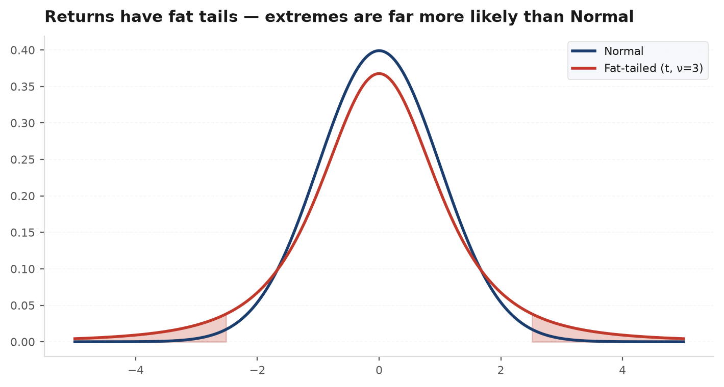
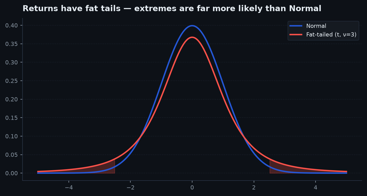
Markets did not read the textbook. Real return distributions are fat-tailed(leptokurtic): the peak is taller and narrower, and — the part that matters — the tails are far heavier than a Normal allows. Those “once every 14,000 years” 5-sigma days show up several times a decade. October 1987 was a ~20-sigma move under a Normal fit; under a Normal it is impossible, yet it happened.

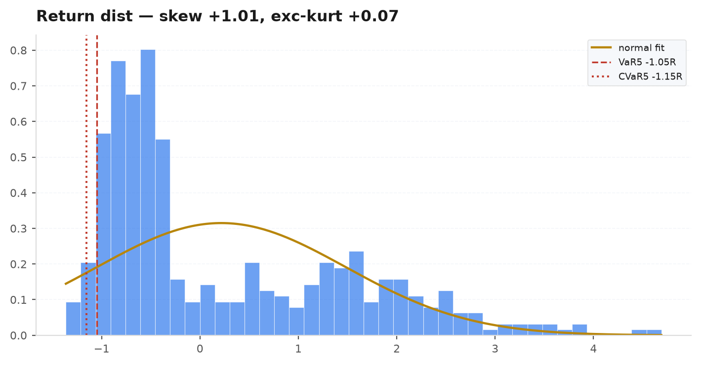
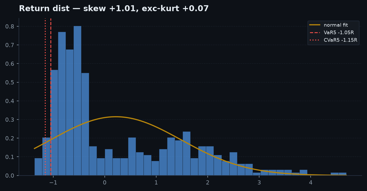
A fat-tailed distribution overlaid on a Normal, showing a taller peak and heavier tails — A fat-tailed return distribution (solid) vs a Normal with the same mean and variance (dashed). More mass in the center and in the extreme tails; less in the shoulders. The tail excess is where blow-ups live.

You can see the same fact in real data. Below is edgekit’s return-distribution chart — a histogram of realised returns with a Normal fit laid over it. The overflowing tail bars are the risk a Normal model would have told you to ignore.

Histogram of realised returns with a fitted Normal overlay showing tail excess — edgekit.viz return distribution: realised returns vs a fitted Normal. The gap in the tails is exactly the risk that Normal-based models understate.

✕Why this is the whole risk-management problem

Nearly every classical risk formula assumes Normality, and every one of them under-estimates tail risk as a result. A model that says ruin is a 1-in-a-million event when it is really 1-in-500 will feel safe right up until it isn’t. Assume fatter tails than your data shows, and stress-test rather than trust a closed-form number.

Skew & kurtosis#

Mean and variance are the first two moments. The next two describe the shape that fat tails live in.

Skewness#

The third standardised moment — the asymmetry of the distribution:

Skew (X) = E [(\frac{X - μ}{σ})^{3}]

Negative skew means a long left tail: many small gains punctuated by rare large losses — the classic shape of short-option and mean-reversion strategies (and it is how a lot of blow-ups feel: fine, fine, fine, catastrophe). Positive skew is the opposite: many small losses and occasional large wins, the signature of trend-following. A Normal has zero skew.

Kurtosis#

The fourth standardised moment — how heavy the tails are:

Kurt (X) = E [(\frac{X - μ}{σ})^{4}]

A Normal has kurtosis 3, so people quote excess kurtosis $Kurt (X) - 3$ : positive means fatter-than-Normal tails. Financial returns routinely show large positive excess kurtosis. High kurtosis is the formal statement of “fat tails.”

✦Read skew before you trust a Sharpe

Two strategies can share a mean and volatility — and so an identical Sharpe — while one has benign positive skew and the other hides a fat left tail. This is precisely why edgekit.metrics insists you report profit factor and MAR beside Sharpe: the higher moments are where Sharpe goes blind.

VaR & CVaR#

Since the tail is where you get hurt, we measure it directly. Value at Risk at confidence $α$ (say 95%) is the loss threshold you only breach $(1 - α)$ of the time — the $α$ -quantile of the loss distribution:

VaR_{α} = in f {ℓ : P (L \leq ℓ) \geq α}

VaR has a notorious flaw: it tells you the threshold you will breach but says nothing about how bad things get once you do. Conditional VaR (also Expected Shortfall) fixes that — it is the average loss in the worst $(1 - α)$ of cases:

CVaR_{α} = E [L ∣ L \geq VaR_{α}]

CVaR is the number to prefer, especially with fat tails: it looks into the tail rather than stopping at its edge. Because both are just quantiles and conditional means of the historical loss series, you estimate them empirically rather than from a Normal formula — which, again, would understate them.

tail_risk.py

import numpy as np

# empirical VaR / CVaR from a return series (no Normal assumption)
losses = -returns                       # losses as positive numbers
var95 = np.quantile(losses, 0.95)       # breached 5% of the time
cvar95 = losses[losses >= var95].mean() # average loss beyond VaR

print(f"95% VaR:  {var95:.3%}")
print(f"95% CVaR: {cvar95:.3%}")        # always >= VaR; the honest tail number

In practice you rarely trust a single historical tail estimate — the worst case in your sample is just the worst case you happened to see. edgekit’s Monte-Carlo tools resample the return stream thousands of times to build a distribution of terminal outcomes and drawdowns, giving you a bootstrapped tail rather than the one lucky (or unlucky) path history handed you. That is the subject of Monte Carlo.

Next: we only ever see a sample of the true distribution, so how much can we trust it? — Statistics for traders.