Statistics for traders

You never see a strategy’s true edge — only a finite sample of trades drawn from it, blurred by noise. Statistics is the discipline of saying how much that sample can be trusted. This is the chapter that explains the single most important sentence in the whole course: you need a lot of trades before a backtest means anything.

Sampling & sampling error#

The true expected return per trade, $μ$ , is a fixed but unknown property of the strategy — the population mean. A backtest gives you a sample of $n$ trades, and from it the sample mean:

x ˉ = \frac{1}{n} i = 1 \sum n x_{i}

$x ˉ$ is our estimate of $μ$ , but it is itself random — run the strategy over a different slice of history and you get a different $x ˉ$ . The gap between your sample estimate and the truth is sampling error. It is not a bug or a bad backtest; it is the irreducible fog that comes from having finite data. The entire job of the next few chapters is to keep that fog from fooling you.

Standard error#

How much does $x ˉ$ wobble from sample to sample? Its standard deviation has a name — the standard error of the mean:

SE (x ˉ) = \frac{σ}{n}

→Derivation — the variance of a sample mean

The sample mean is a sum scaled by $1/ n$ . Pull the constant out of the variance (which costs a square):

Var (x ˉ) = Var (\frac{1}{n} i = 1 \sum n x_{i}) = \frac{1}{n ^{2}} Var (i = 1 \sum n x_{i})

If the trades are independent, the variance of the sum is the sum of the variances (no covariance terms), and each has the same $σ^{2}$ :

= \frac{1}{n ^{2}} i = 1 \sum n Var (x_{i}) = \frac{1}{n ^{2}} (n σ^{2}) = \frac{σ ^{2}}{n}

Take the square root to get back to the units of the mean: $SE (x ˉ) = σ / n$ . The $n$ is not magic — it is the square root of the $n^{2}$ -vs- $n$ mismatch between scaling and adding. ■

!The independence caveat

The clean

n σ^{2}

step needed independence. If trades overlap or share a regime they are positively correlated, the dropped covariance terms are positive, and the true SE is larger than

σ / n

— your effective sample size is smaller than your trade count. Correlated returns make you more confident than you deserve to be.

Read this formula slowly, because it governs everything. The uncertainty in your estimate shrinks with the square root of the number of trades — not linearly. To halve your uncertainty you need four times as many trades. To cut it by ten, a hundred times as many. This is why a strategy with 30 trades tells you almost nothing and one with 1,000 tells you something real.

Trades n	√n	SE relative to n = 25
25	5	1.00× (baseline)
100	10	0.50× (half the error)
400	20	0.25×
2,500	50	0.10×

✦Scenario: is a +0.2R edge over 30 trades real?

Your ORB backtest shows an average of

+ 0.2 R

per trade over

n = 30

trades, with the usual per-trade spread of about

σ = 1 R

. The standard error of that mean is

σ / n = 1/ 30 \approx 0.18 R

— almost as big as the edge itself. Your measured

+ 0.2 R

is only about

0.2/0.18 \approx 1.1

standard errors from zero, so a true edge of exactly zero would routinely throw off a sample this good. Now run the same strategy long enough to log

n = 400

trades at the same

+ 0.2 R

: the standard error drops to

1/ 400 = 0.05 R

, the edge is now

4

standard errors out, and zero becomes very hard to believe. The number did not change — the evidence did, and only

n

moved.

!This is the deep reason few-trade backtests lie

A strategy with a big historical return but only 20 or 30 trades has an enormous standard error — its true edge could easily be zero. Impressive-looking, statistically empty results almost always trace back to a small

n

. When you read a backtest, look at the trade count before the return.

The law of large numbers#

Before the mean can be Normal, it first has to land on the truth at all. That guarantee is the law of large numbers (LLN): as the number of trades grows, the sample mean converges to the true mean.

x ˉ_{n} n \to \infty μ

It is the mathematical form of “let the edge play out.” A positive-expectancy strategy is not promised to win on any given trade — only that, averaged over enough of them, the realised mean is pulled toward $μ$ . The LLN is why an edge is worth having; it is also why it needs volume to materialise.

Chebyshev’s inequality — a distribution-free proof#

We can prove the LLN and get a usable bound in one stroke with Chebyshev’s inequality, which holds for any distribution with finite variance — no Normality, no thin tails required:

P (∣ X - μ ∣ \geq k σ) \leq \frac{1}{k ^{2}}

→Proof sketch + how it forces the LLN

Chebyshev follows from Markov’s inequality applied to $(X - μ)^{2}$ : since that quantity is non-negative with mean $σ^{2}$ , the probability it exceeds $(k σ)^{2}$ is at most $σ^{2} / (k σ)^{2} = 1/ k^{2}$ . The event $(X - μ)^{2} \geq (k σ)^{2}$ is the same as $∣ X - μ ∣ \geq k σ$ , giving the bound.

Now apply it to the sample mean, which has standard deviation $σ / n$ . For any fixed tolerance $ε > 0$ ,

P (∣ x ˉ_{n} - μ ∣ \geq ε) \leq \frac{σ ^{2}}{n ε ^{2}} n \to \infty 0

The probability of the sample mean straying from $μ$ by any margin vanishes as $n \to \infty$ — that is exactly convergence, and the LLN. ■

✦Why it matters for trading

Chebyshev is deliberately loose (it wastes nothing on tail shape), which makes it the honest tool when returns are fat-tailed and the Normal “95% within 2σ” rule cannot be trusted. It guarantees at least

1 - 1/ k^{2}

of outcomes fall within

k

standard deviations — e.g.

\geq 75%

within 2σ,

\geq 88.9%

within 3σ — no matter how ugly the distribution. A worst-case bound you can actually rely on.

The central limit theorem#

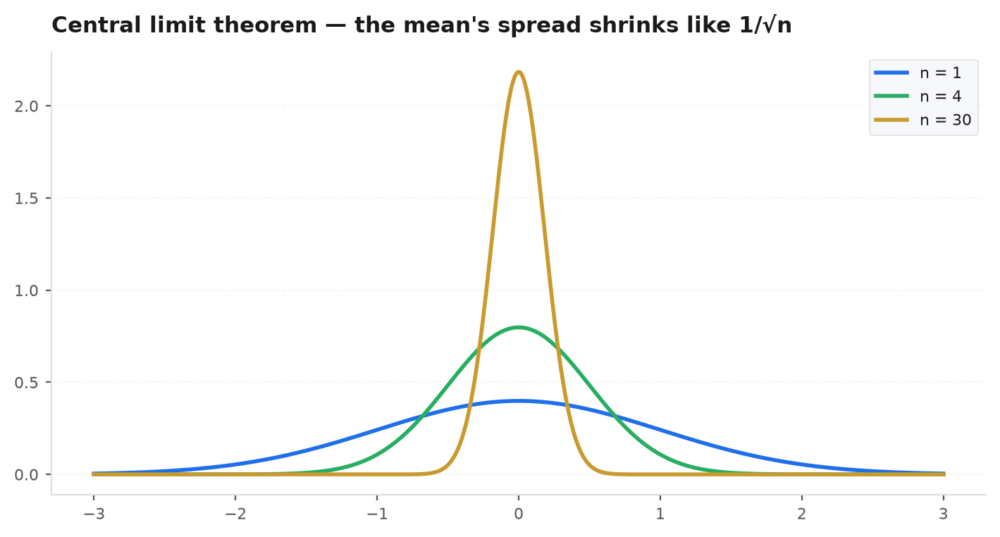
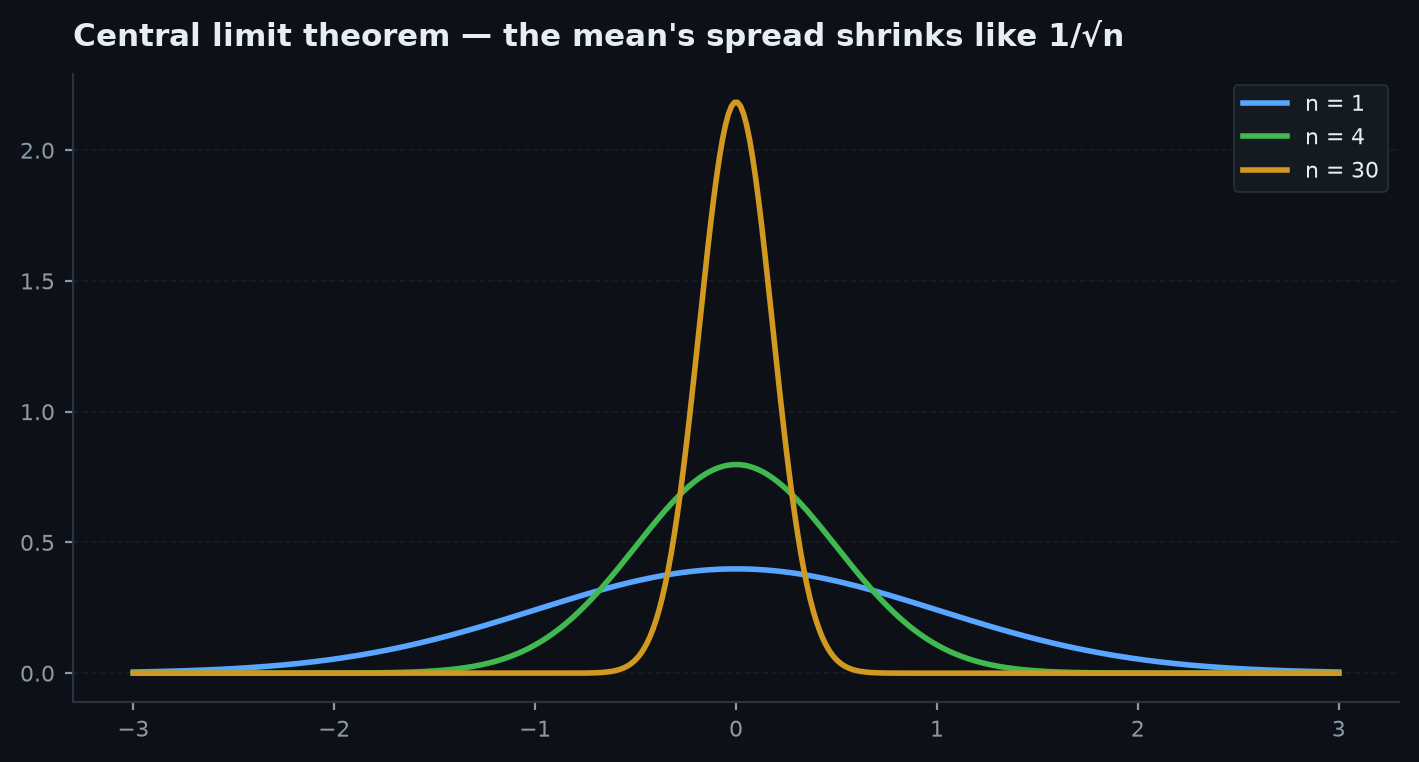
Why can we use $σ / n$ and reason with the bell curve, when individual returns are fat-tailed and nothing like Normal? Because of the central limit theorem (CLT): the distribution of the sample mean of $n$ independent draws approaches a Normal as $n$ grows — regardless of the shape of the underlying distribution.

x ˉ n \to \infty N (μ, \frac{σ ^{2}}{n})

The individual trades can be as skewed and fat-tailed as markets truly are; average enough of them and the average settles into a tidy bell curve centered on the truth, tightening as $n$ rises. That is what licenses every confidence interval and hypothesis test that follows.

→Sketch — why Normal, and the √n rate

The mechanism is a competition of moments. Standardise the sample mean as $Z_{n} = n (x ˉ - μ) / σ$ . Its skew shrinks like $1/ n$ and its excess kurtosis like $1/ n$ , so as $n$ grows every deviation from a bell shape is scrubbed away and only the mean and variance survive — the defining property of a Normal. (The rigorous version matches characteristic functions.) Note the scaling: we multiplied by $n$ to keep $Z_{n}$ from collapsing to a point, which is the same statement as $SE = σ / n$ : the mean concentrates, and the width of what is left of its distribution closes at rate $1/ n$ — quadruple the trades to halve the noise.

Sampling distributions of the mean tightening into a bell curve as sample size grows — The central limit theorem in action: even from a skewed source distribution, the sampling distribution of the mean becomes Normal and narrows as n grows — width shrinks like 1/√n.

→Fat tails slow the CLT down

The CLT is asymptotic, and fat tails make it converge slowly — a single monster trade can still dominate a modest sample. So the CLT is a reason to gather many trades, not an excuse to trust a small sample because “means are Normal.” When in doubt, resample empirically (bootstrap) instead of leaning on the formula — see Monte Carlo.

Confidence intervals#

A point estimate $x ˉ$ without a range is a false precision. A confidence interval puts a band around it. Using the CLT and the 95% rule for a Normal, the 95% interval for the true mean is:

x ˉ \pm 1.96 \cdot \frac{σ}{n}

→Derivation — inverting the standardised mean

From the CLT, $x ˉ \sim N (μ, σ^{2} / n)$ , so the standardised mean is a standard Normal:

Z = \frac{x ˉ - μ}{σ / n} \sim N (0, 1)

The value $z = 1.96$ is chosen so a standard Normal lands inside $[- z, z]$ with probability 0.95. So with 95% probability,

- 1.96 \leq \frac{x ˉ - μ}{σ / n} \leq 1.96

Multiply through by $σ / n$ and rearrange to isolate $μ$ :

x ˉ - 1.96 \frac{σ}{n} \leq μ \leq x ˉ + 1.96 \frac{σ}{n} . ■

For a general confidence level, swap 1.96 for the matching Normal quantile $z_{1 - α /2}$ (2.58 for 99%).

The interpretation is subtle and worth getting right: it does notsay “there is a 95% probability the truth is in this interval.” It says that if you repeated the whole experiment many times, 95% of the intervals you construct this way would contain the true $μ$ . It is a statement about the reliability of the procedure, not about this one interval.

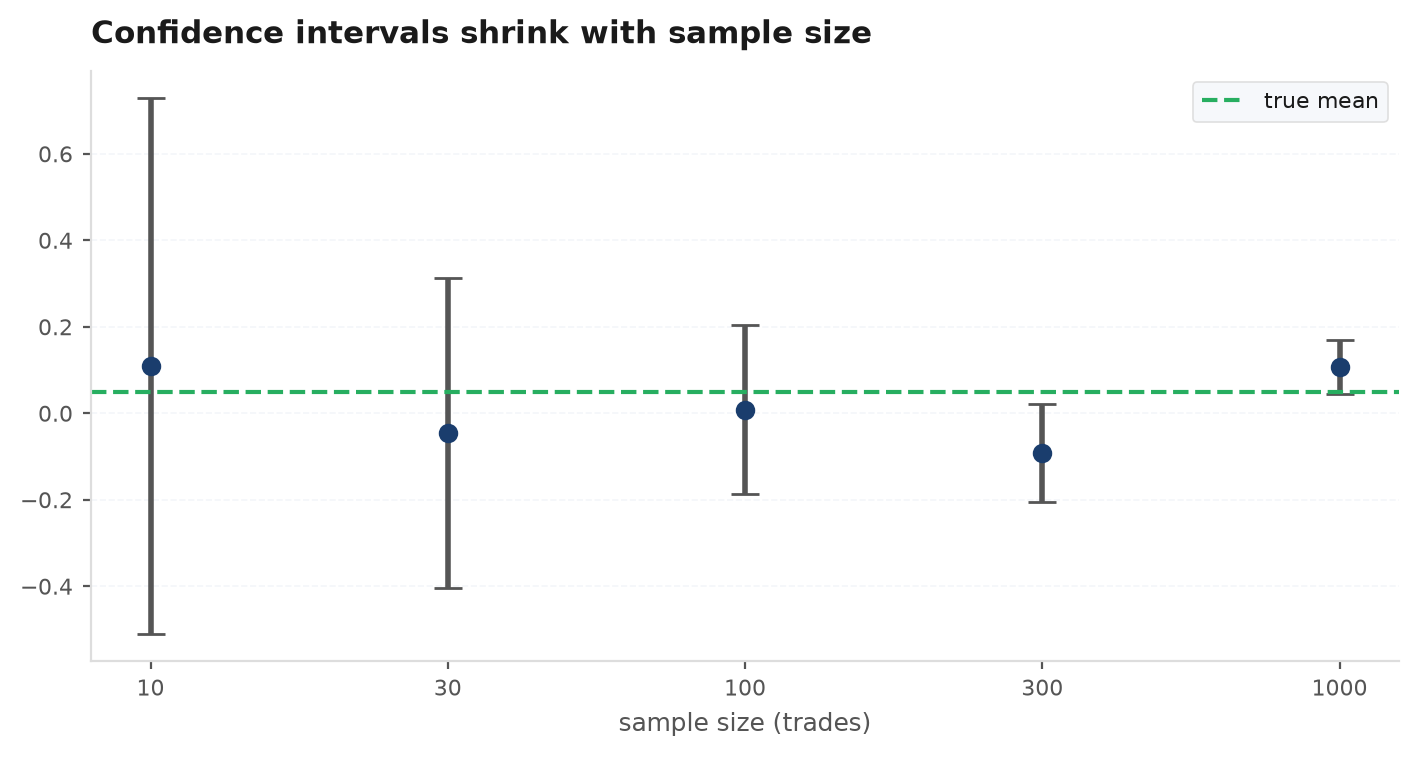
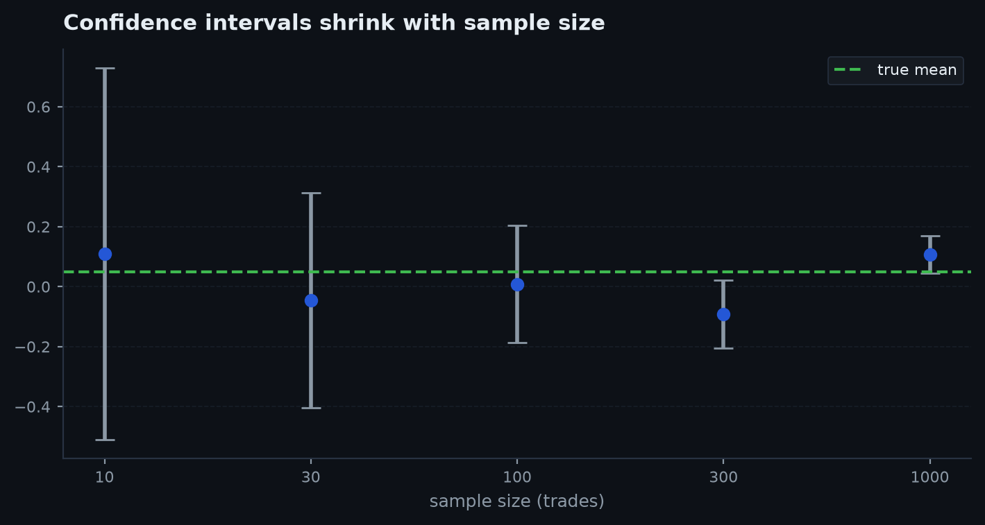
A point estimate with a 95% confidence band, and repeated intervals most of which cover the true value — 95% confidence intervals from repeated samples. About 1 in 20 misses the true mean (dashed line). Wider samples (smaller n) give wider bands — the honest picture of what a backtest can and cannot claim.

The practical payoff: the same estimated edge is convincing with a narrow band and meaningless with a band that straddles zero. When you compute a strategy’s expectancy, always ask whether zero is inside its interval. If it is, you do not yet have evidence of an edge — only a hint.

edge_ci.py

import numpy as np
from edgekit import trade_stats

st = trade_stats(trades.r)            # per-trade R-multiples
r = np.asarray(trades.r, float)
n = r.size

mean = r.mean()
se = r.std(ddof=1) / np.sqrt(n)       # standard error of the mean
lo, hi = mean - 1.96 * se, mean + 1.96 * se

print(f"expectancy: {st['ev_r']:.3f}R  (n={n})")
print(f"95% CI: [{lo:.3f}, {hi:.3f}]R")
if lo <= 0 <= hi:
    print("zero is inside the band -> no statistical evidence of edge yet")

Hypothesis testing & p-values#

Confidence intervals and hypothesis tests are two sides of the same coin. A hypothesis test formalises the skeptic’s question: could this result just be luck?

The null hypothesis#

You start by assuming the boring explanation — the null hypothesis $H_{0}$ : the strategy has no edge, its true expectancy is zero, every apparent profit is noise. Your result is only interesting if the data makes this null look untenable. You never prove the null false; you either reject it or fail to reject it.

What a p-value actually means#

The p-value is the probability of seeing a result at least as extreme as the one you got, if the null hypothesis were true:

p = P (result at least this extreme ∣ H_{0} true)

A small p (conventionally $p < 0.05$ ) means “a no-edge world would rarely produce something this good, so the no-edge story is hard to believe.” Be precise about what it is not: p is not the probability that your strategy has no edge, and it is not the probability the result is due to chance. It is a conditional probability assuming the null — a measure of how surprised a skeptic should be, nothing more.

Type I and Type II error#

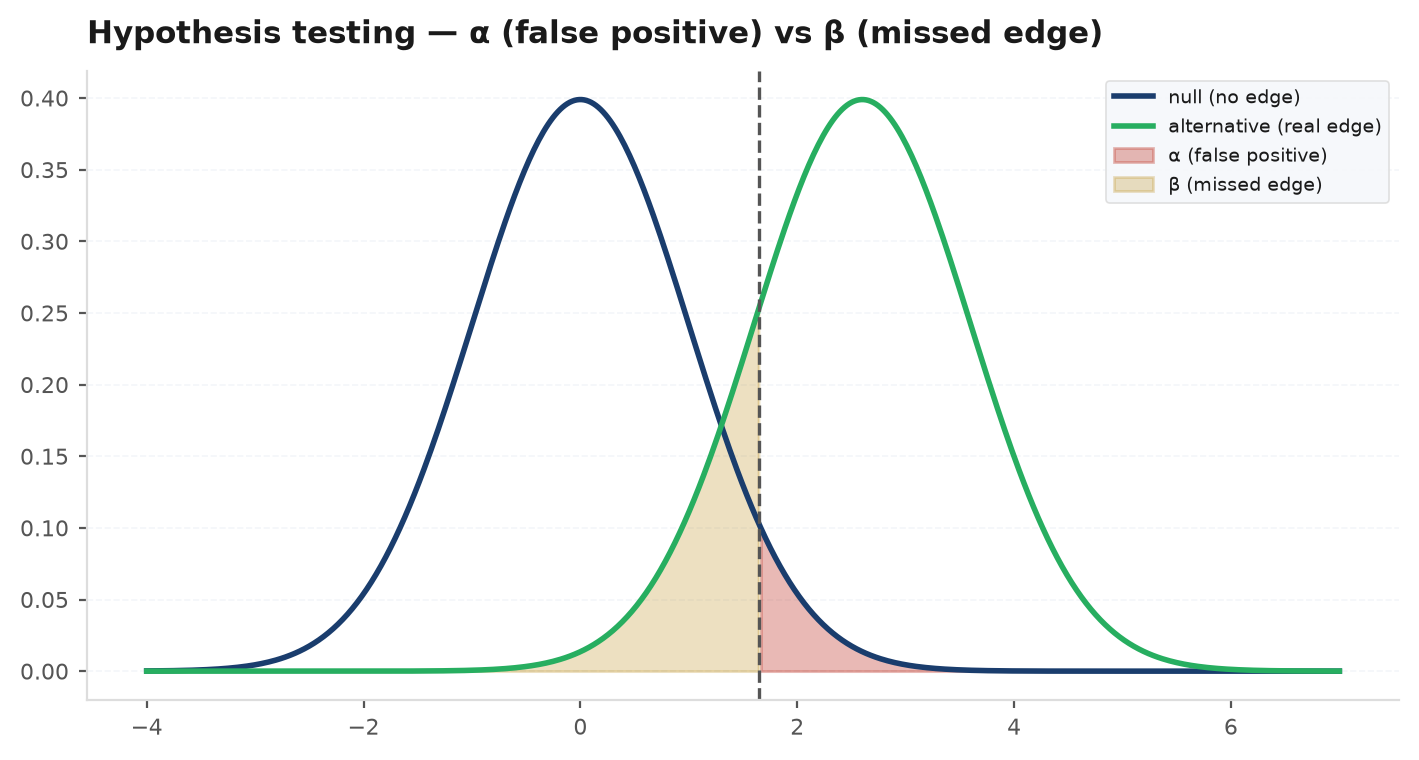
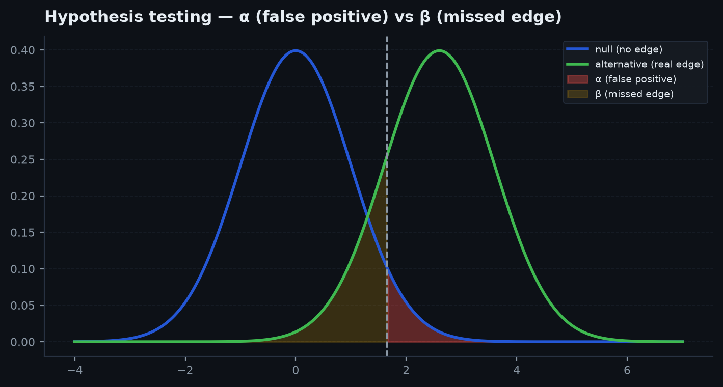
A test can be wrong two ways. A Type I error (false positive) is rejecting a true null — deploying a strategy that has no edge. A Type II error (false negative) is failing to reject a false null — discarding a strategy that really works. Their probabilities have standard names:

α = P (reject H_{0} ∣ H_{0} true), β = P (fail to reject H_{0} ∣ H_{0} false)

Your significance threshold is $α$ — set it to 0.05 and you accept a 5% false-positive rate per test. The quantity $1 - β$ is the power: the chance of catching a real edge when there is one. The two trade off — demanding a smaller $α$ raises $β$ unless you add data — and the lever that improves both at once is a larger $n$ , which tightens $σ / n$ and separates the two hypotheses.

Null and alternative distributions with the alpha false-positive region and beta missed-edge region shaded — The two error types made visible. Under the null (no edge) the shaded α tail is where you falsely 'discover' an edge; under the alternative (real edge) the shaded β region is where you miss it. Moving the threshold trades one for the other — only more data (which pulls the curves apart) shrinks both at once.

✦Why it matters for trading

A trader’s Type I error costs real money (a dead strategy that draws down); a Type II error is only opportunity cost. That asymmetry is why the gauntlet is deliberately strict — better to reject a few good strategies than to fund a fluke. But run enough tests at

α = 0.05

and false positives become near-certain: 20 independent no-edge tests yield roughly one “significant” result on average. That is the multiple-testing problem below.

!Significant does not mean large, or real

With enough trades a trivially small edge becomes “statistically significant,” and — the far worse trap — if you test enough strategies, some will clear

p < 0.05

by pure luck. A single p-value from a single test is a weak defense. This is exactly the multiple-testing problem that Why most backtests lie is built around.

Because market returns violate the neat assumptions behind textbook t-tests (independence, Normality), edgekit does not lean on a closed-form p-value. It uses a permutation test: shuffle the data to build the null distribution empirically, then read off where the real result falls. The p-value becomes a simple count:

p = \frac{1 + # { s _{i}^{*} \geq s }}{N + 1}

where $s$ is your real statistic and $s_{i}^{*}$ are the $N$ statistics from shuffled (no-edge) data. This is edgekit.validation.mcpt, the decisive step of the gauntlet.

✦Scenario: reading a permutation p-value off your backtest

Your strategy’s real backtest posts a profit factor of

s = 1.40

. You shuffle the returns

N = 1000

times to destroy any real ordering-based edge, re-run each shuffle, and record its profit factor

s_{i}^{*}

. Suppose 82 of those edge-free shuffles happened to score

1.40

or better. Then

p = (1 + 82) / (1000 + 1) \approx 0.083

— an 8% chance a no-edge world fakes a result this good, which does not clear the usual 0.05 bar. Had only 4 shuffles beaten it,

p \approx 0.005

, and the no-edge story would be genuinely hard to defend. Same PF of 1.40 either way; what the permutation test measures is how easily randomness reproduces it.

mcpt.py

from edgekit.validation import mcpt, bootstrap_rng

# real_stat = your strategy's observed metric (e.g. profit factor)
# null_fn() = one draw of that metric under a shuffled, edge-free world
p = mcpt(real_stat, null_fn, n=1000, rng=bootstrap_rng())
print(f"permutation p = {p:.3f}")   # small p => the null struggles to fake this

Why we need many trades — the through-line#

Everything in this chapter is the same fact stated four ways:

Standard error is $σ / n$ — few trades, huge uncertainty.
The CLT only tightens the estimate as $n$ grows.
Confidence intervals shrink like $1/ n$ .
A p-value needs enough data to distinguish edge from noise.

A strategy with 40 trades and a gorgeous equity curve is, statistically, a rumor. One with 700 trades that survives a permutation test is a claim you can act on. It is why the strategies worth deploying tend to be the ones that trade often enough to accumulate evidence — and why every backtest in this course reports its trade count as prominently as its return.

Next: now we can define edge precisely and ask how many trades it takes to show up — The math of edge.