The math of edge

“Edge” is not a vibe — it is a number. It is the expected value of one trade, measured in units of risk. This chapter defines it precisely, shows why it is invisible until you have taken many trades, and then confronts the harder question the beginner never asks: given a real edge, how much should you bet? The answers are less aggressive than intuition suggests.

R-multiples — the unit of edge#

Dollars are a bad unit for comparing trades, because a $500 win on a $5,000 risk is nothing like a $500 win on a $50 risk. The fix is the R-multiple: express every outcome as a multiple of the amount you risked on that trade ( $1 R$ = your initial stop distance in dollars).

R = \frac{profit or loss on the trade}{dollars risked at entry}

A trade stopped out for its full risk is $- 1 R$ ; one that makes three times its risk is $+ 3 R$ . R-multiples make trades of different sizes and different instruments directly comparable, and they are the native language of edgekit.metrics — trade_stats takes an array of per-trade R and gives you everything else.

→Why the R-multiple is the right unit

Dividing by dollars-risked normalises every trade to the same scale, so the per-trade outcomes

R_{1}, R_{2}, \dots

become draws from one common distribution rather than apples-and-oranges dollar figures. That single move is what makes the expectation

E [R]

, the variance, and every probability statement in this chapter well-defined: you cannot average a distribution that changes units every trade. R-multiples turn a messy trade log into a clean sample from a random variable.

Expectancy#

Suppose a strategy wins with probability $p$ , and on a win it makes $W$ (in R) while on a loss it gives back $L$ (in R, positive). Its expectancy is the expected R per trade:

E [R] = p W - (1 - p) L

✦Derivation — expectancy is just E[·] of a two-outcome variable

Model one trade as a random variable $R$ that takes the value $+ W$ with probability $p$ and $- L$ with probability $1 - p$ . By the definition of expected value — the probability-weighted sum of the outcomes —

E [R] = x \sum x P (R = x) = (+ W) p + (- L) (1 - p) = p W - (1 - p) L .

Short proof via linearity. Write the outcome with two indicator variables, $R = W 1_{win} - L 1_{loss}$ , where $1_{win} = 1$ on a win and $0$ otherwise. The expectation of an indicator is just the probability of its event, $E [1_{win}] = P (win) = p$ . Linearity of expectation — $E [a X + bY] = a E [X] + b E [Y]$ , which holds with no independence assumption — then gives $E [R] = W E [1_{win}] - L E [1_{loss}] = p W - (1 - p) L$ .

Why it matters for trading. The formula is exact for a single trade and assumes nothing about independence or identical distribution — those enter only when you average many trades (below). So expectancy is well-defined even for a strategy whose trades are correlated or whose payoff shape drifts; it is the one number that tells you whether the game is worth playing at all.

This is the single most important formula in trading. It is just the expected value from Probability & distributions applied to a trade. If $E [R] > 0$ you have an edge; if $E [R] \leq 0$ no amount of clever money management can save you. edgekit reports this as ev_r.

Win rate p	Avg win W	Avg loss L	Expectancy E[R]	Edge?
0.40	2.0R	1.0R	+0.20R	Yes — low win rate, big winners
0.60	1.0R	1.0R	+0.20R	Yes — same edge, different shape
0.70	0.5R	1.5R	−0.10R	No — high win rate, still loses
0.50	1.0R	1.0R	0.00R	Coin flip — no edge

✦Scenario: the first row, in dollars, over 100 trades

Take the top row —

p = 0.40

W = 2 R

L = 1 R

, so

E [R] = + 0.20 R

. Trade it on a $100,000 account risking

R = $500

per trade, so each trade is worth

+ $1, 000

on a win and

- $500

on a loss, and the average trade earns

0.20 \times $500 = $100

. Over 100 trades your expected profit is

$10, 000

. But you win only 40% of them, so you will string together losing runs — six losses in a row (

- $3, 000

) is unremarkable for a 40%-win system. The edge is real and the drawdowns are real at the same time; the

+ $100

/trade only shows up once the losers and the fat winners have both had their turn.

→Win rate alone tells you nothing

A 70%-win strategy can be a money-loser and a 40%-win strategy a winner. Only the combination of win rate and payoff — i.e. expectancy — decides. Beginners chase high win rates; the math cares about

E [R]

Payoff ratio#

The payoff ratio $b = W / L$ is the average win divided by the average loss. It lets you find the breakeven win rate for any payoff — the win rate at which $E [R] = 0$ :

p_{breakeven} = \frac{1}{1 + b} = \frac{L}{W + L}

✦Derivation — set the expectancy to zero and solve

Breakeven is the win rate at which the edge vanishes, so set $E [R] = p W - (1 - p) L = 0$ and solve for $p$ :

p W = (1 - p) L \Rightarrow p W + p L = L \Rightarrow p (W + L) = L \Rightarrow p = \frac{L}{W + L} = \frac{1}{1 + W / L} = \frac{1}{1 + b} .

Why it matters for trading. This is the bar the real hit rate must clear after costs. Costs act by shrinking every $W$ and enlarging every $L$ , which lowers $b$ and raises $p_{breakeven}$ — the reason a gross edge so often turns into a net loss. Choosing a target R is therefore not a preference; it is a commitment to beat a specific, computable win rate.

With a 2:1 payoff you only need to win a third of the time to break even; with a 1:2 payoff you need to win two-thirds. This is the trade-off every strategy design negotiates: wider targets buy you a lower required win rate but a lower hit rate to go with it. In edgekit, an ORB(or_bars=30, target_r=2.0) is picking a 2R payoff and therefore a ~33% breakeven — everything hinges on whether the real hit rate clears it once costs are paid.

The law of large numbers#

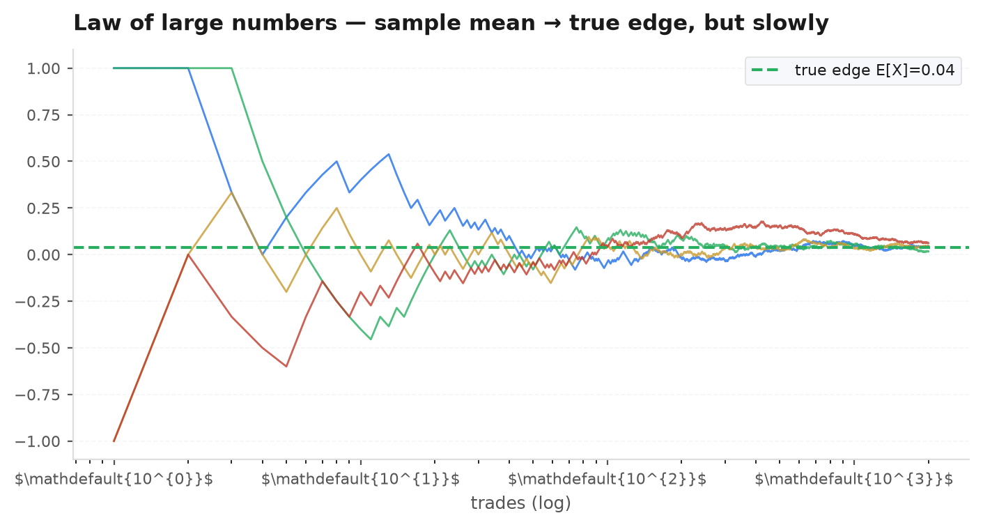
Expectancy is a statement about the average of many trades — and here is the catch that ruins undercapitalised traders: over a small number of trades, expectancy is invisible. The law of large numbers says the sample average converges to the true expectancy only as the number of trades grows:

R ˉ_{n} = \frac{1}{n} i = 1 \sum n R_{i} n \to \infty E [R]

→Proof sketch — why it converges, and how slowly

Assume the trades are independent with common mean $E [R] = μ$ and variance $σ^{2}$ . Linearity gives $E [R ˉ_{n}] = μ$ (the sample average is unbiased), and because variance of independent sums adds,

Var (R ˉ_{n}) = \frac{1}{n ^{2}} i = 1 \sum n Var (R_{i}) = \frac{σ ^{2}}{n} n \to \infty 0.

A random variable with a fixed mean and a variance collapsing to zero concentrates on that mean (Chebyshev: $P (∣ R ˉ_{n} - μ ∣ \geq ε) \leq σ^{2} / (n ε^{2}) \to 0$ ). That is the weak law. Why it matters for trading: the standard error of your measured edge shrinks only as $σ / n$ — the square-root-of-n law. Halving your uncertainty needs four times the trades; a $+ 0.2 R$ edge with per-trade noise $σ \approx 1 R$ needs on the order of a hundred trades before the signal clears the noise. This is precisely why a losing month tells you almost nothing.

The word converges hides a slow, noisy reality. A genuine $+ 0.2 R$ edge can sit underwater for dozens of trades in a row; a losing streak of 8–10 is routine even for a good system. Early on, luck dominates skill — the running average staggers around before it settles. This is the mathematical reason a losing month tells you almost nothing.

A running average of trade R-multiples slowly converging toward the true expectancy — Law of large numbers: the running average edge (noisy line) only settles onto its true expectancy (dashed) after many trades. Early swings are pure sampling noise, not signal.

!Edge and survival are different problems

A positive expectancy guarantees you win eventually. It says nothing about surviving the drawdowns along the way — and if a losing streak wipes you out first, the eventual edge never arrives. That is why edge (this section) and sizing (the next) are two separate questions, and both must be answered.

Random walks and the martingale baseline#

What does no edge look like in the language of probability? It is a martingale: a process whose best forecast of its next value, given everything you know, is simply its current value.

E [P_{t + 1} ∣ P_{t}, P_{t - 1}, \dots] = P_{t} ⟺ E [next return ∣ past] = 0.

A price that is a pure random walk is a martingale, and it is a theorem (the optional-stopping theorem) that no trading rule — no stop, target, or clever entry timing — can manufacture positive expectancy from a martingale: every strategy inherits $E [R] = 0$ before costs, and a loss after them. An edge is precisely a departure from the martingale property: $E [R] > 0$ means the game, in your direction, is a submartingale — the conditional expectation drifts up, not flat. Everything in this course is an attempt to establish, honestly, that a given series is not a martingale.

→Why it matters for trading

The martingale is the null hypothesis you are always testing against. The permutation test in the next chapterworks by literally shuffling your data into a martingale and asking whether your edge could have come from that. If a strategy’s returns are indistinguishable from a driftless random walk, its beautiful backtest is measuring luck, not signal.

The Kelly criterion#

Given a real edge, how much of your capital should you risk per trade? Bet too little and you leave growth on the table; bet too much and volatility drag (from Returns & compounding) — or ruin — eats you alive. The Kelly criterion is the bet fraction that maximises the long-run geometric growth rate. For a payoff ratio $b$ and win probability $p$ :

f^{*} = \frac{p ( b + 1 ) - 1}{b}

✦Derivation — maximise expected log-growth

Why log growth? Because wealth compounds multiplicatively: after $n$ bets your capital is a product of per-bet multipliers, and the log turns that product into a sum whose long-run average is governed by the law of large numbers. Maximising the expected log return per bet, $G (f) = E [ln (1 + f X)]$ , therefore maximises the long-rungeometric growth rate. Let the per-unit outcome be $X = + b$ on a win (probability $p$ ) and $X = - 1$ on a loss (probability $1 - p$ ), and stake fraction $f$ :

G (f) = p ln (1 + f b) + (1 - p) ln (1 - f) .

Differentiate and set to zero (the game is concave in $f$ , so this is the max):

G^{'} (f) = \frac{p b}{1 + f b} - \frac{1 - p}{1 - f} = 0.

p b (1 - f) = (1 - p) (1 + f b) \Rightarrow p b - p b f = (1 - p) + (1 - p) b f .

Collect the $f$ terms — the right-side $b f$ factors combine:

p b - (1 - p) = b f [p + (1 - p)] = b f \Rightarrow f^{*} = \frac{p b - ( 1 - p )}{b} = \frac{p ( b + 1 ) - 1}{b} .

The second derivative $G^{''} (f) = - \frac{p b ^{2}}{( 1 + f b ) ^{2}} - \frac{1 - p}{( 1 - f ) ^{2}} < 0$ everywhere, confirming $f^{*}$ is a maximum, not a saddle. Notice the numerator $p b - (1 - p)$ is exactly the expectancy per unit staked: no edge, no bet.

!Why fractional Kelly — the variance of log-growth is huge

Full Kelly maximises the expected log-growth, but it says nothing about its variance, which at $f^{*}$ is punishingly large — full-Kelly equity swings routinely halve the account. Because $G (f)$ is concave, a second-order expansion around the optimum,

G (f) \approx G (f^{*}) - \frac{1}{2} ∣ G^{''} (f^{*}) ∣ (f - f^{*})^{2},

shows growth falls off only quadratically as you back away from $f^{*}$ while volatility falls linearly. That asymmetry is the whole case for fractional Kelly: betting $\frac{1}{2} f^{*}$ keeps roughly three-quarters of the growth for about half the volatility. Since $p$ and $b$ are themselvesestimated with the sampling error above, betting a fraction also hedges the very real chance you have over-estimated your edge.

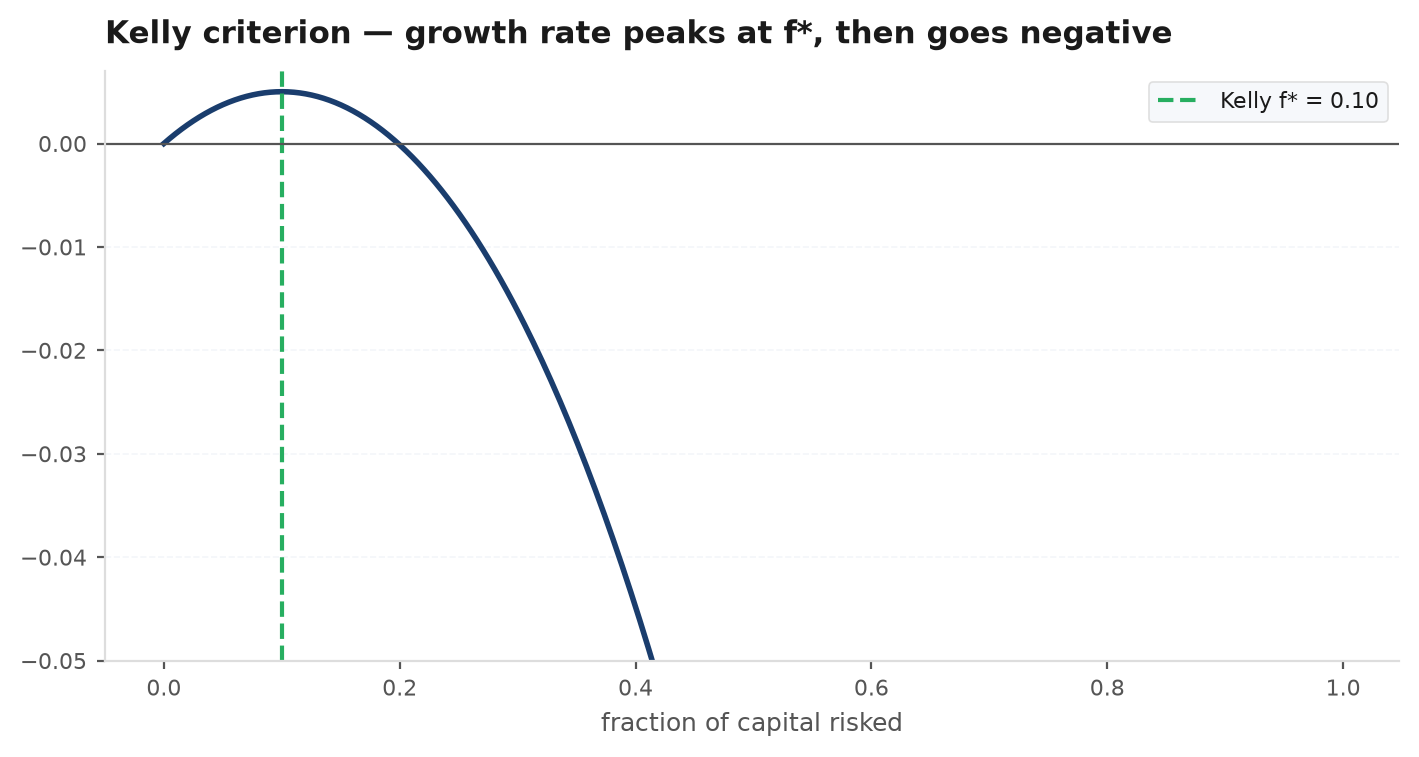
The numerator is just the expectancy per unit staked, so Kelly scales your bet with your edge and shrinks it with the payoff’s riskiness. A strategy with $p = 0.55$ and $b = 1$ gives $f^{*} = 0.10$ — risk 10% of capital per bet to grow fastest. The growth-rate curve peaks at $f^{*}$ and falls off on both sides; push past it and growth actually turns negative despite the positive edge.

Long-run growth rate as a function of bet fraction, peaking at the Kelly fraction and going negative when over-betting — Growth rate vs bet fraction. It peaks at f*, and crucially the curve is asymmetric — over-betting past ~2f* drives long-run growth below zero even though every individual bet has positive expectancy.

✦Scenario: a coin-flip edge, sized three ways

You have an even-money strategy (

b = 1

) that wins

p = 0.55

of the time. Full Kelly says

f^{*} = \frac{0.55 ( 1 + 1 ) - 1}{1} = 0.10

— risk 10% of the account per bet to grow fastest. On $100,000 that is a $10,000 stake per trade, and the theory promises the maximum long-run growth rate. It also promises equity swings that routinely halve the account, and if your true

p

is really 0.53 (you over-estimated), 10% is now over-betting the real edge. Half-Kelly —

5%

, a $5,000 stake — keeps roughly three-quarters of the growth for about half the volatility. That is the trade nearly every professional takes, and it is why edgekit sizes to a drawdown budget rather than betting a full, fragile point-estimate of

f^{*}

Why full-Kelly is too aggressive#

Nobody serious bets full Kelly. Three reasons, all fatal in practice:

The curve is flat on top but a cliff on the right. Half-Kelly captures about 75% of the growth for roughly half the volatility — a wonderful trade. Over-betting is punished far more harshly than under-betting.
Your edge is estimated, not known. $p$ and $b$ come from a finite sample with the standard error of the last chapter. If you have over-estimated your edge, full-Kelly on the true (smaller) edge is already over-betting.
Full-Kelly drawdowns are brutal. The expected worst drawdown at full Kelly routinely exceeds 50% — deeper than almost any real account (or prop-firm rule) can tolerate.

The standard practice is fractional Kelly — a quarter to a half of $f^{*}$ . edgekit sidesteps the fragile point-estimate of Kelly entirely for deployment: rather than bet a fraction of a guessed edge, edgekit.sizing sizes against a hard drawdown budget, which is the constraint that actually binds a real account.

edge_to_size.py

from edgekit import trade_stats, sizing

# 1) measure the edge, in R
st = trade_stats(trades.r, dates=trades.date)
print(st["ev_r"], st["win_rate"], st["pf"])   # is E[R] > 0 with enough trades?

# 2) size to a drawdown budget rather than a full-Kelly guess
res = sizing.size_to_dd(daily_r, dd_budget=0.095, account=100_000)
res["dollar_per_r"]   # dollars to risk per 1R so historical max DD == 9.5%
res["binding"]        # which constraint set the size

Risk of ruin#

The flip side of Kelly. Risk of ruin is the probability that a string of losses drags your account below a threshold you cannot come back from — before the edge has time to pay out. For a simplified even-money game with win probability $p$ and $N$ units of capital, the classic gambler’s-ruin result is:

P_{ruin} = (\frac{1 - p}{p})^{N}

✦Derivation — first-step analysis of the gambler's ruin

Track capital in whole units and let $r_{i}$ be the probability of eventual ruin (hitting $0$ ) starting from $i$ units, with win probability $p$ and loss probability $q = 1 - p$ per bet. Condition on the first bet — this is first-step analysis, an application of the law of total probability:

r_{i} = p r_{i + 1} + q r_{i - 1}, r_{0} = 1.

This linear recurrence has characteristic equation $p x^{2} - x + q = 0$ , whose roots are $x = 1$ and $x = q / p$ . The general solution is therefore $r_{i} = A + B (q / p)^{i}$ . With a positive edge $(p > q)$ the ruin probability must stay bounded and tend to $0$ as capital grows, forcing $A = 0$ ; the boundary $r_{0} = 1$ forces $B = 1$ . Hence $r_{i} = (q / p)^{i}$ , and starting from $N$ units,

P_{ruin} = (\frac{q}{p})^{N} = (\frac{1 - p}{p})^{N} .

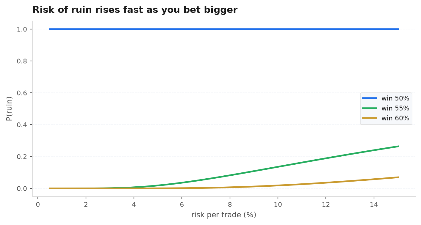
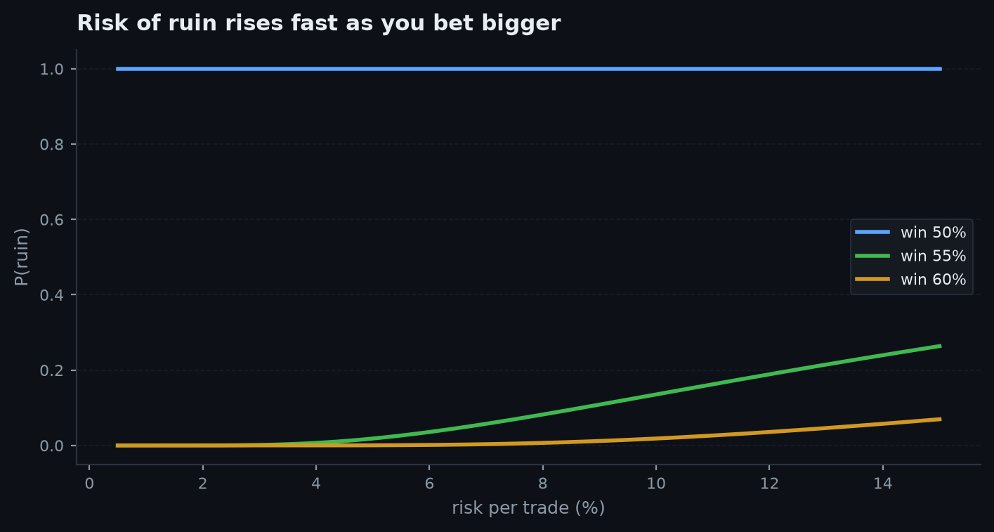
Why it matters for trading. A drawdown limit — a prop-firm rule, or the level below which you quit — is exactly a lower absorbing barrier on this walk. The exponent $N$ is how many units of risk your capital represents, and you set it with bet size: risk 1% per trade and $N = 100$ ; risk 10% and $N = 10$ . Because ruin decays geometrically in $N$ , over-betting shrinks the exponent and drives $(q / p)^{N} \to 1$ — a positive edge with too large a bet is almost sure to be ruined before the law of large numbers can pay it out. Edge sets the base $q / p < 1$ ; sizing sets the exponent — and the exponent wins.

Two levers control it: the size of your edge ( $p$ above 0.5) and how many units of risk your capital represents ( $N$ , which you set by bet size). Even a solid edge combined with an over-sized bet gives a frightening probability of ruin — and once ruined, the positive expectancy is worthless because you are no longer in the game.

✦Scenario: same edge, bet size decides survival

Keep the winning edge

p = 0.55

(so

q / p = 0.45/0.55 \approx 0.818

) and treat “ruin” as losing the whole account. If you risk 1% per trade, your capital is

N = 100

units and the ruin probability is

0.81 8^{100}

— around

1 0^{- 9}

, effectively zero. Crank the bet to 10% per trade and now

N = 10

0.81 8^{10} \approx 0.13

— a 13% chance of blowing up despite the identical, genuinely positive edge. Push to 20% (

N = 5

) and it climbs to

0.81 8^{5} \approx 0.37

. The signal never changed; the exponent did. Sizing, not edge, is what keeps you in the game long enough for the edge to pay.

Risk of ruin rising sharply as bet size per trade increases, for a fixed positive edge — Risk of ruin against risk-per-trade for a fixed positive edge. Small bets keep ruin near zero; past a point the same edge is almost certain to blow up. Sizing, not signal, decides survival.

✦The whole message in one line

Edge decides whether you win in the long run; sizing decides whether you live long enough to see it. A positive expectancy and a bet size that keeps risk-of-ruin near zero are both required — neither substitutes for the other. This is the bridge into Position sizing.

Next: we have the math to define and size an edge — so why do so many backtests show edges that evaporate live? Why most backtests lie.