Copulas & dependence
Every portfolio decision rests on a model of how assets move together. The number almost everyone uses — the Pearson correlation — measures only linear co-movement and is blind to exactly the dependence that destroys portfolios: joint crashes. This chapter separates the two questions a joint distribution answers (how does each asset behave alone, and how are they wired together), states Sklar’s theorem that makes the separation exact, and shows why a Gaussian dependence model has zero tail dependence — the mathematical reason diversification evaporates precisely when you need it.
Two portfolios can both report “correlation 0.3” and be utterly different animals. In one, the assets co-move mildly all the time. In the other, they are nearly independent on calm days and lock together on crash days. Same correlation coefficient, wildly different risk: the second portfolio’s diversification is a fair-weather friend. Correlation compresses an entire two-dimensional dependence structure into one number, and the compression throws away the corner of the distribution where accounts die. Copulas are the tool that keeps the structure.
Where Pearson correlation fails#
Pearson’s is the covariance normalised to :
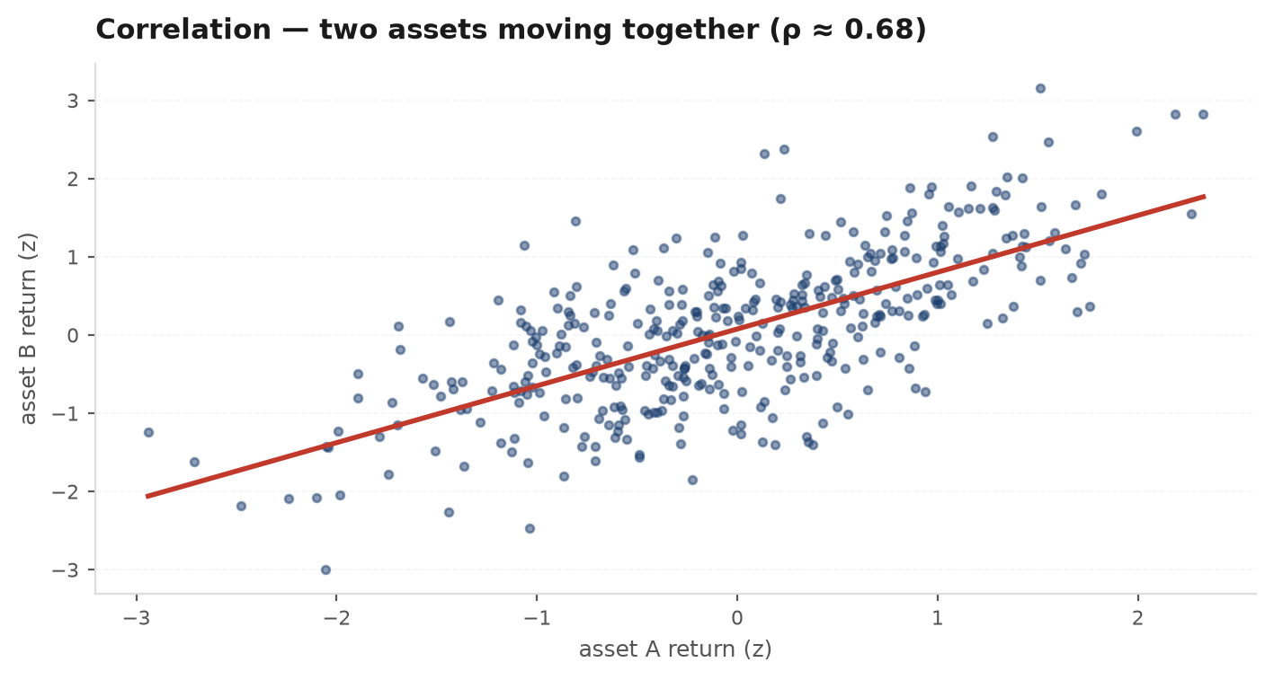
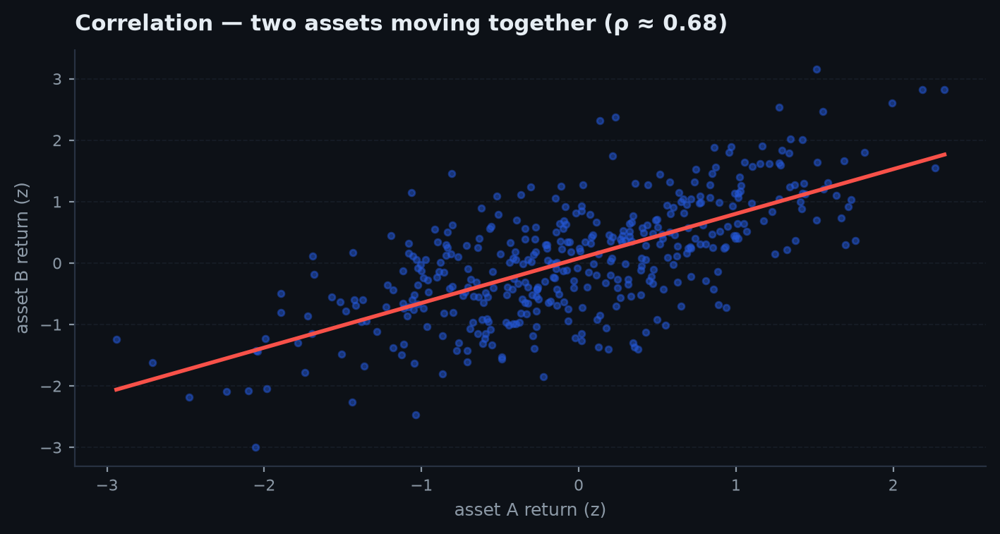
It measures the strength of the best linear fit between and — nothing more. Three failure modes matter at the desk:
- Nonlinearity. If with symmetric around zero, then exactly — perfect deterministic dependence, zero measured correlation. Like Anscombe’s quartet for regression, radically different joint scatters can share one correlation number.
- Non-ellipticity. Interpreting as “the” dependence is only justified for elliptical distributions (multivariate normal, multivariate t). Real return pairs are not elliptical: their dependence is asymmetric, stronger on the downside.
- Tail blindness. is dominated by the mass of ordinary days. Two assets can have modest full-sample correlation and still crash together with near certainty — the statistic barely notices, because crash days are rare in the average it computes.
Rank correlations: Kendall and Spearman#
A first repair is to measure dependence on ranks rather than values. Kendall’s tau asks: for a random pair of observations, are they concordant (both up or both down together) or discordant?
Spearman’s rho is the Pearson correlation of the ranks. Both are invariant under any strictly increasing transform of either variable: replace with or and does not move, because ranks do not move. That invariance is the tell: rank correlations depend only on the dependence structure, not on the marginal distributions — they are properties of the copula, defined next.
import edgekit as ek

rets = prices.pct_change().dropna()          # DataFrame, one column per strategy

tau = ek.dependence.kendall_matrix(rets)     # rank-based dependence, robust to marginals
mst = ek.dependence.corr_mst(rets)           # minimum spanning tree on d = sqrt(2(1 - rho))
for a, b, dist in mst:
    print(f"{a} -- {b}: {dist:.3f}")         # the backbone of the correlation structure
Sklar’s theorem — marginals versus wiring#
The central result of dependence modelling says the split we have been gesturing at is exact. A copula is a joint CDF on whose marginals are uniform — a pure dependence structure with the individual distributions stripped out.
Let be a joint CDF with continuous marginals and . The probability-integral transform says and are each uniform on : for ,
Define — the joint CDF of the transformed pair, which by construction has uniform marginals, i.e. is a copula. Substituting back:
Sklar’s theorem: every joint distribution is its marginals composed with a copula, and (for continuous marginals) the copula is unique. The marginals say how each asset behaves alone; the copula is the wiring diagram between them. You can mix and match — fat-tailed marginals with Gaussian wiring, or thin marginals with crash-prone wiring — and the risk consequences are entirely different.
Gaussian versus t-copula#
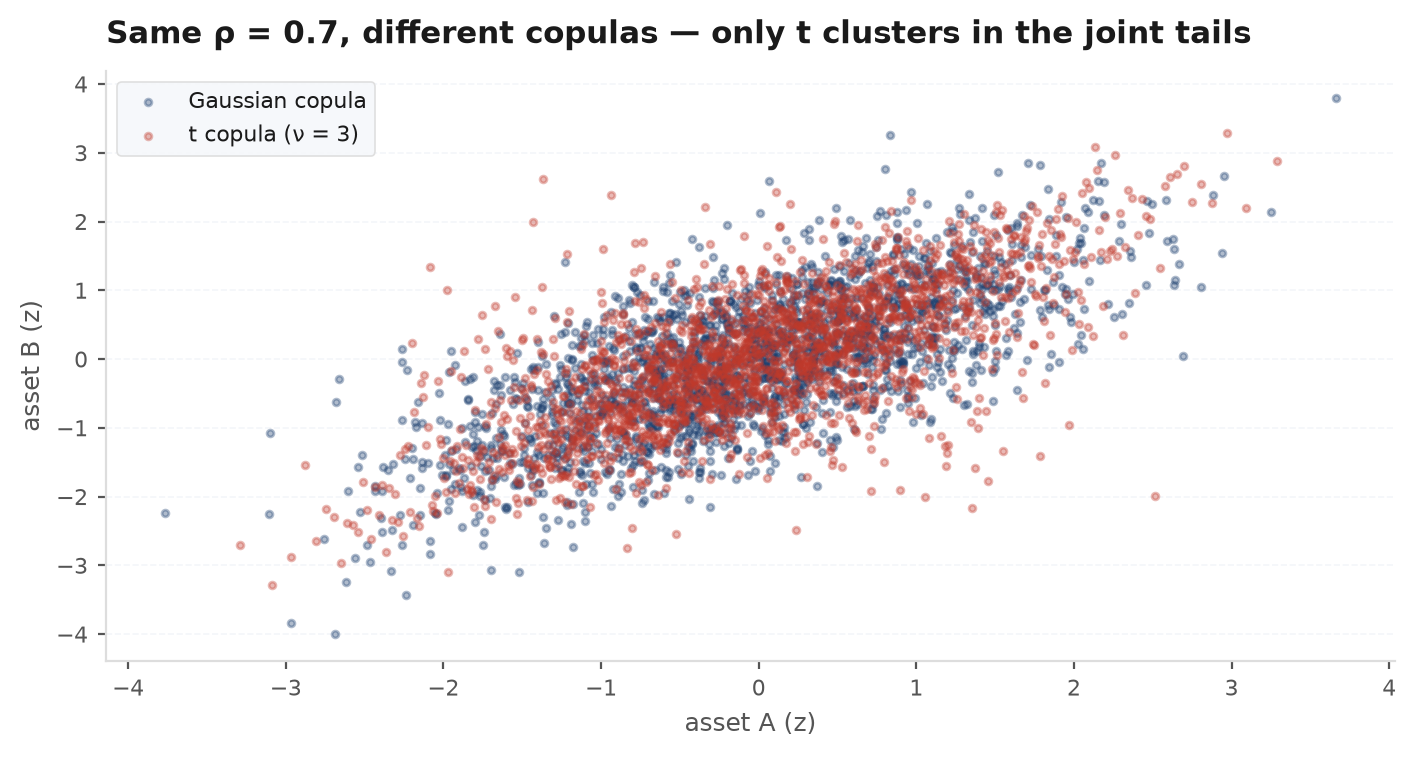
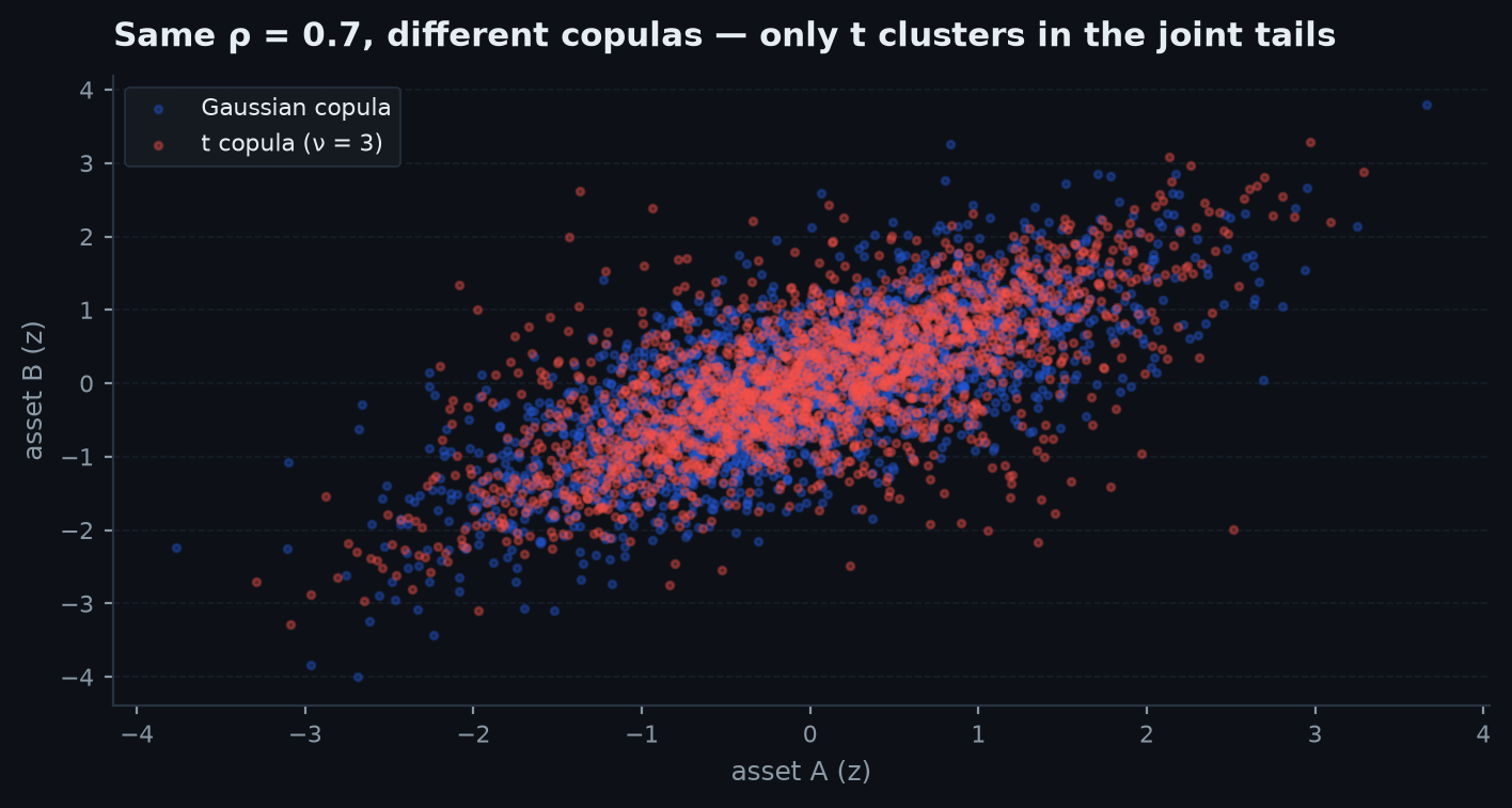
The two workhorse copulas both come from elliptical families. The Gaussian copula is the dependence structure of a multivariate normal: transform correlated normals through the normal CDF, . The t-copula does the same with a multivariate Student-t: divide the normals by a shared draw first. That shared divisor is the whole story — when the chi-square draw is small, every component is inflated at once, manufacturing joint extremes that the Gaussian cannot produce.
Tail dependence — the killer fact#
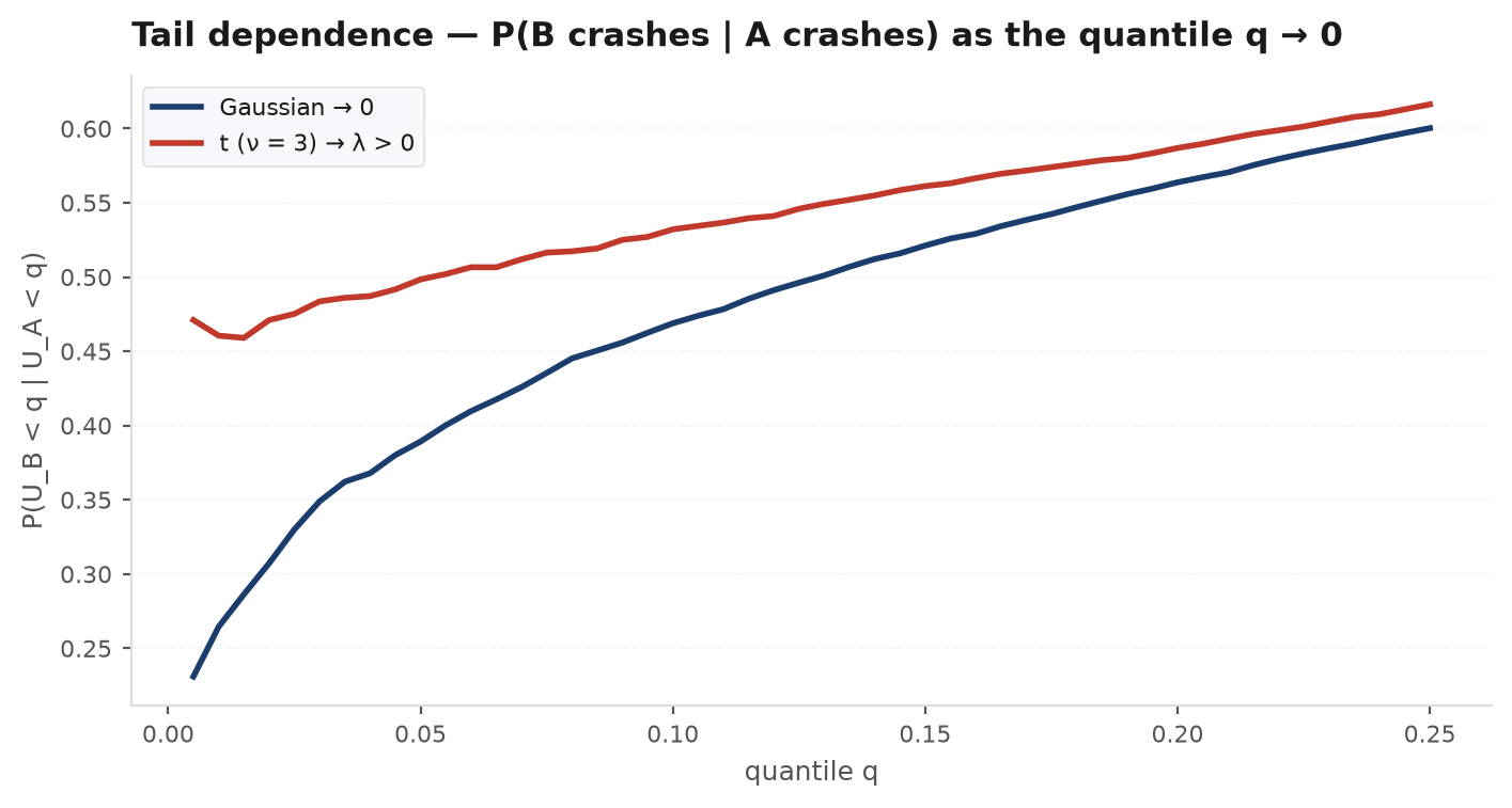
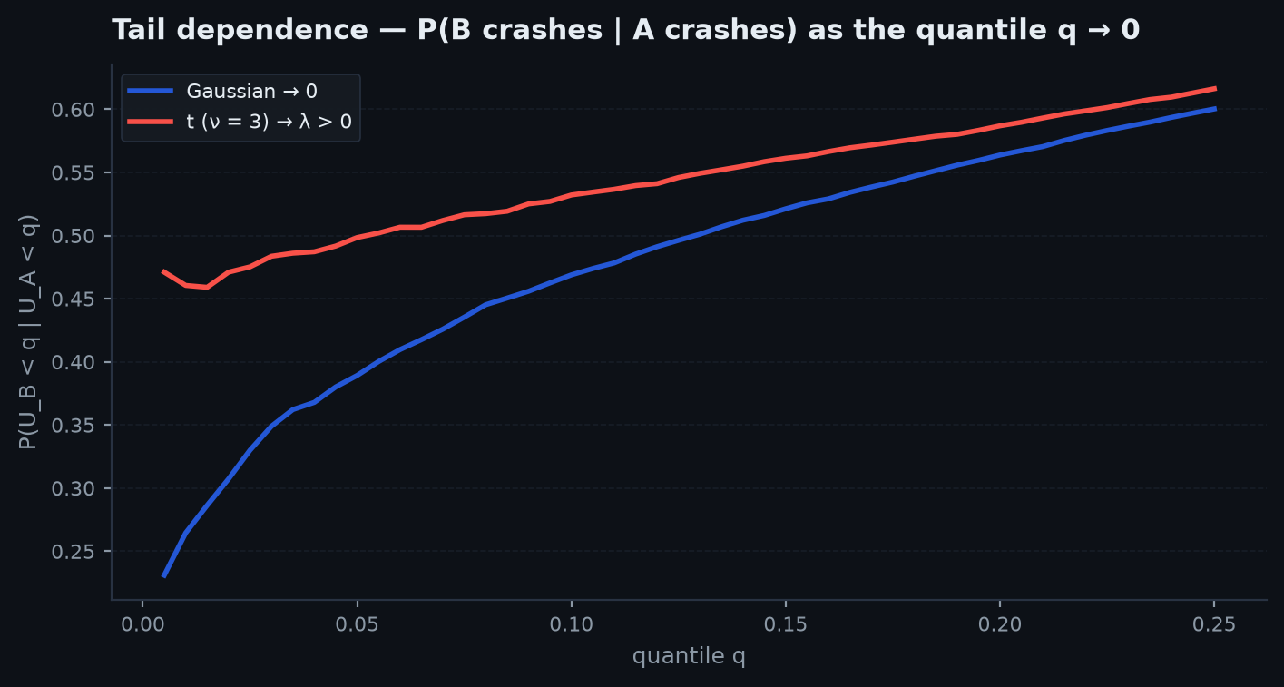
The property that separates them has a name. Lower tail dependence is the probability that one asset is in its worst -fraction of outcomes given the other is:
with defined symmetrically in the upper corner. For the Gaussian copula with any correlation :
Zero. Not small — zero. Under Gaussian dependence, conditional on one asset having an extreme day, the probability the other one does too vanishes as you go further into the tail. The t-copula, by contrast, has strictly positive tail dependence for every : the closed form is , where is the Student-t CDF — increasing in , decreasing in the degrees of freedom , and positive even at .
Worked scenario — two strategies, calm correlation 0.3#
Take two strategies whose daily returns show Pearson correlation over a calm sample. You allocate half to each, expecting crash days to partially offset. How often do both land in their worst 5% of days at the same time?
Under independence the co-crash probability would be of days. Under a Gaussian copula at , simulation gives roughly — dependence helps the corner a bit, but the conditional probability still fades toward zero at more extreme quantiles. Under a t-copula with and the same , the closed form gives — and unlike the Gaussian’s conditional probability, this one does notdecay: on the very worst days, one strategy tanking implies roughly a one-in-six chance the other tanks with it, however far into the tail you look. At the 1% threshold the co-crash rate under the t-copula is several times the Gaussian’s. Your “diversified” book is one book on exactly the days diversification was bought for.
import edgekit as ek

rets = strat_returns.dropna()                          # DataFrame: two strategy return columns

# Fit both wirings to the same data (correlation from Kendall tau: rho = sin(pi/2 * tau))
gauss = ek.dependence.fit_copula(rets, family="gaussian")
tcop = ek.dependence.fit_copula(rets, family="t", df=4.0)

# Empirical tail dependence in the historical sample
td = ek.dependence.tail_dependence(rets.iloc[:, 0], rets.iloc[:, 1], q=0.05)
print(td)                                              # {"lower": ..., "upper": ...}

# Simulate 100k joint days under each wiring and compare co-crash rates
u_g = ek.dependence.sample_copula(gauss, n=100_000)    # uniforms in (0,1)
u_t = ek.dependence.sample_copula(tcop, n=100_000)
co_crash_g = ((u_g < 0.05).all(axis=1)).mean()
co_crash_t = ((u_t < 0.05).all(axis=1)).mean()
print(f"co-crash 5%: gaussian {co_crash_g:.4f}, t {co_crash_t:.4f}")
The workflow generalises: fit marginals however you like (empirical, fat-tailed), fit the copula on ranks, then stress the portfolio under t-wiring even if calm-period statistics look Gaussian. The copula samples are uniforms — push them through each strategy’s inverse marginal CDF to get joint return scenarios for the Monte-Carlo engine.
Assumptions versus reality#
| Correlation-matrix thinking assumes | Reality | Consequence |
|---|---|---|
| Dependence is fully captured by ρ | Dependence is a structure (a copula), not a scalar | Same ρ can hide benign or lethal wiring |
| Elliptical (Gaussian) joint shape | Asymmetric, crash-skewed dependence | Downside co-movement underestimated |
| Tail dependence λ = 0 | Empirical λ_L > 0 for most risk assets | Joint crashes far likelier than modelled |
| ρ is stable across regimes | Correlations spike toward 1 in stress | Diversification vanishes when needed most |
fit_copulamaps Kendall’s tau to the correlation parameter via rather than using the Pearson estimate.Next: copulas describe how assets crash together; the marginals still need a model of how extreme a single crash can be. That is the domain of extreme value theory — the statistics of maxima and tails, where the Gaussian is not just inaccurate but structurally wrong. Extreme value theory.