Extreme value theory

The central limit theorem governs averages, and averages are not what kill trading accounts — single worst days are. Extreme value theory is the branch of statistics built for the tail itself: it says what the distribution of maxima and threshold exceedances must look like, gives the tail a one-parameter fingerprint $ξ$ , and lets you estimate a 99.9% VaR from a sample that has never seen a 1-in-1000 day. This chapter builds the two limit theorems, the Hill estimator and its honesty problem, and the EVT formulas for VaR and expected shortfall.

✦Intuition — why the CLT says nothing about your worst day

The CLT is a statement about sums: add enough independent returns and the total is approximately normal near its centre. Convergence in the tails is agonisingly slow, and more fundamentally, your risk is not a sum — it is a maximum. “What is my worst day in the next four years?” is a question about $M_{n} = max (X_{1}, \dots, X_{n})$ , and the CLT is silent about it. The right question is: does the maximum, suitably rescaled, converge to anything? It does — and the answer is one of the cleanest results in probability.

Fisher–Tippett–Gnedenko: three tails, one family#

Let $X_{1}, \dots, X_{n}$ be i.i.d. losses and $M_{n}$ their maximum. The Fisher–Tippett–Gnedenko theorem says: if there exist normalising sequences $a_{n} > 0, b_{n}$ such that $(M_{n} - b_{n}) / a_{n}$ converges to a non-degenerate distribution, that distribution must be the generalised extreme value (GEV) family:

G_{ξ} (x) = exp [- (1 + ξ x)^{- 1/ ξ}], 1 + ξ x > 0,

with the $ξ = 0$ case read as the limit $exp (- e^{- x})$ . One parameter sorts every distribution into three domains of attraction:

Gumbel ( $ξ = 0$ ): light, exponential-type tails — the normal and log-normal live here. Extremes exist at every size but become rare very fast.
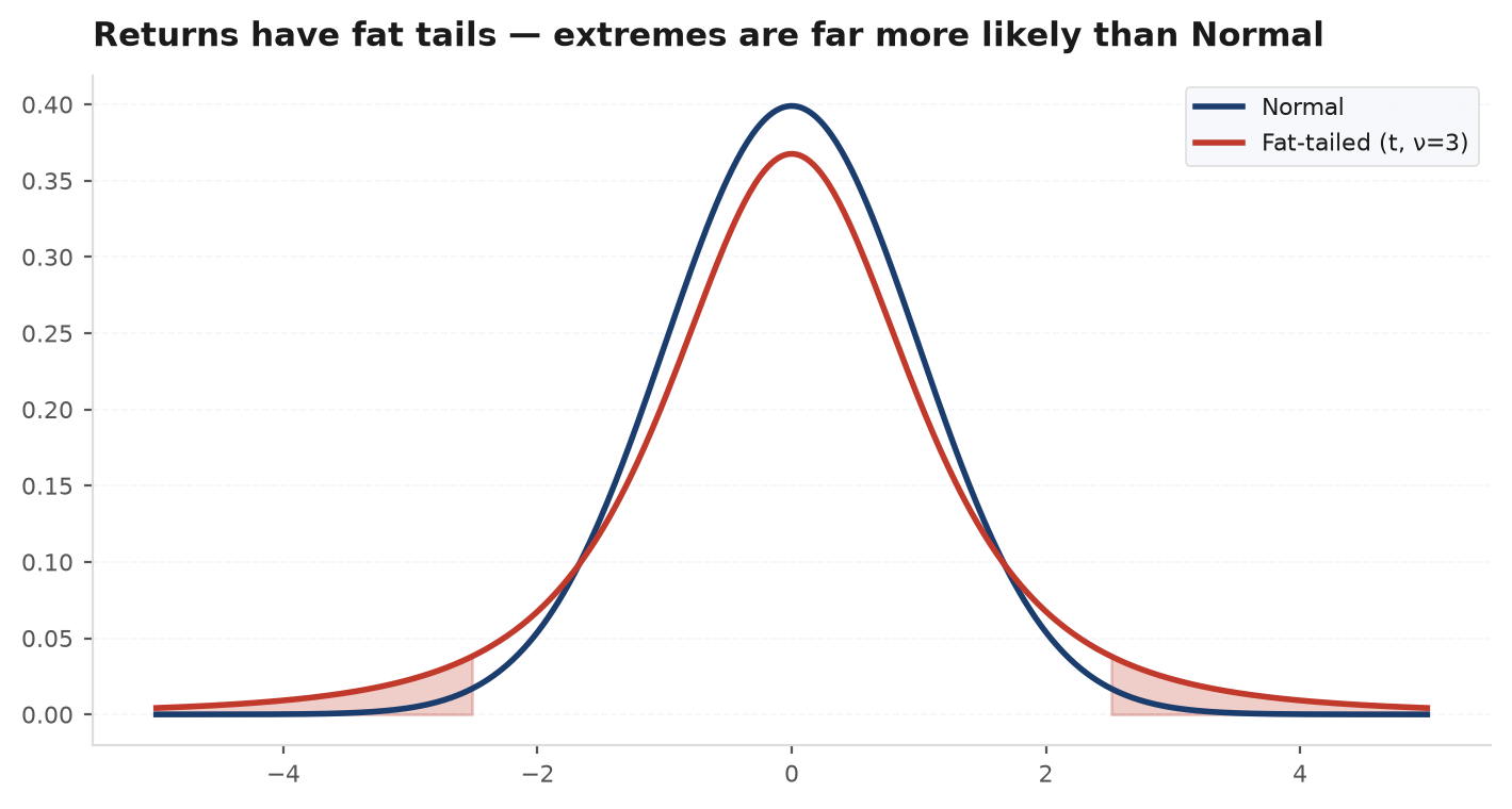
Fréchet ( $ξ > 0$ ): heavy power-law tails — Student-t, Pareto, and, empirically, financial returns. Extremes are polynomially likely; some moments are infinite.
Weibull ( $ξ < 0$ ): bounded tails with a hard upper endpoint — relevant for capped payoffs, not for market losses.

This is the tail-side analogue of the CLT: just as sums forget their parent distribution and become normal, maxima forget theirs and become GEV. The parent only survives through one number, $ξ$ .

A normal density overlaid with a fat-tailed return distribution on log scale, the fat tail sitting orders of magnitude above the Gaussian in the extremes — Why the domain matters: on a log scale, a fat (Fréchet-domain) tail sits orders of magnitude above the Gaussian at extreme levels. A risk model that assumes xi = 0 when the data has xi > 0 is not slightly wrong in the tail — it is wrong by factors of hundreds.

Peaks over threshold and the GPD#

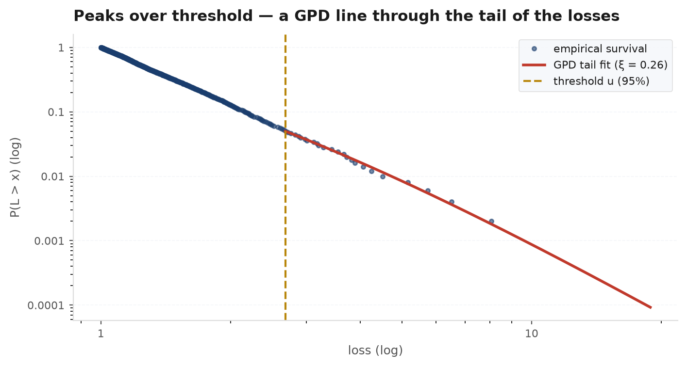
Fitting a GEV to block maxima (one worst day per year, say) wastes data. The modern route keeps every loss beyond a high threshold $u$ and models the excesses $X - u$ . The Pickands–Balkema–de Haan theorem is the licence: for any distribution in a GEV domain of attraction, as $u$ rises the conditional distribution of excesses converges to the generalised Pareto distribution (GPD),

P [X - u \leq y ∣ X > u] ⟶ G_{ξ, β} (y) = 1 - (1 + \frac{ξ y}{β})^{- 1/ ξ},

with scale $β > 0$ and the same shape $ξ$ as the GEV. So the recipe — peaks over threshold (POT) — is: pick $u$ (a high sample quantile, e.g. the 95th), collect the exceedances, fit $(ξ, β)$ , and you own a parametric model of the tail beyond your data.

Empirical survival function of large losses on log-log axes with a fitted generalised Pareto tail extending smoothly beyond the largest observed loss — A GPD fitted to losses beyond the 95% threshold. The fitted curve tracks the empirical tail through the data and then keeps going — a principled extrapolation to loss levels the sample never reached, which is exactly what a 99.9% VaR requires.

→ξ is the tail's fingerprint — and it kills moments

For

ξ > 0

the GPD tail decays like a power law,

P [X > x] \sim x^{- 1/ ξ}

, so moments of order

\geq 1/ ξ

are infinite. At

ξ = 0.5

the variance does not exist; at

ξ = 1

even the mean is gone. Equity index returns typically fit around

ξ \approx 0.2 - 0.4

— variance exists, but the fourth moment (kurtosis) is on the edge, which is why sample kurtosis never converges and why backtest statistics built on it are so unstable.

Block maxima or threshold exceedances?#

The two theorems suggest two workflows, and the choice is mostly settled in POT’s favour for financial data:

Block maxima (GEV):split the sample into blocks (years), keep each block’s worst day, fit the GEV to those maxima. Clean theory, brutal data efficiency — 8 years of daily data yields 8 observations, and the second-worst day of a bad year is discarded even if it dwarfs the worst day of a calm year.
Peaks over threshold (GPD): keep every loss beyond $u$ — typically 5% of the sample rather than one point per year. Same shape parameter, an order of magnitude more tail data, and a direct route to VaR via the survival-function decomposition below.

The price POT pays is the threshold choice: too low and the GPD limit has not kicked in (bias), too high and the fit starves (variance). It is the same bias-variance dial as the Hill estimator’s $k$ , and the honest response is the same — show the estimate’s sensitivity to the dial, not a single number.

The Hill estimator — and Hill-plot honesty#

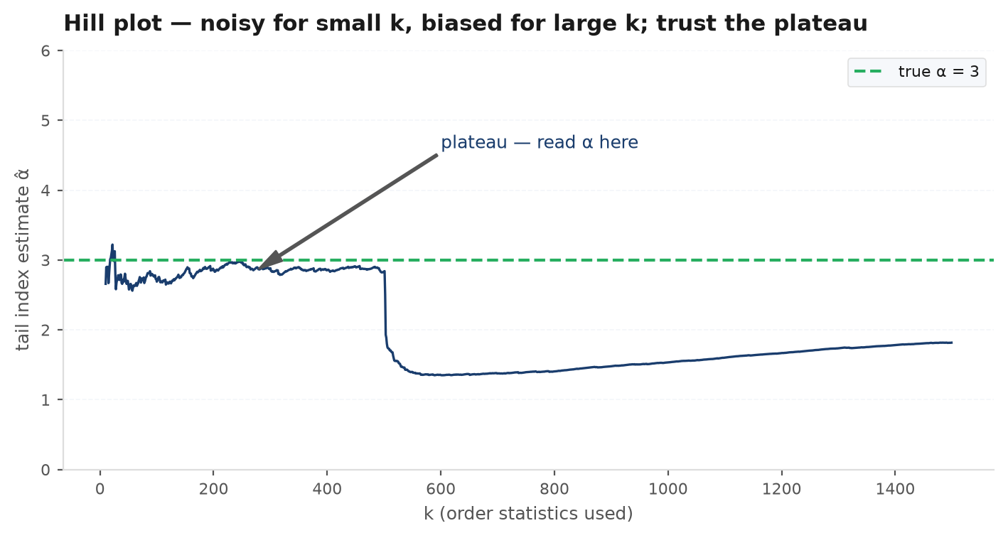
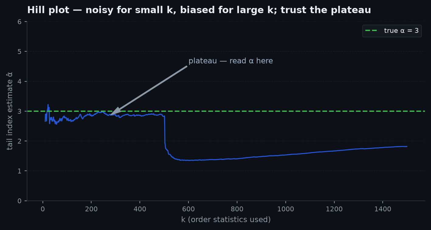
For Fréchet-domain data there is a beautifully direct estimator of the tail index $α = 1/ ξ$ . Sort the losses, $X_{(1)} \geq X_{(2)} \geq \dots$ , take the top $k$ , and average the log-spacings:

α^_{Hill} = [\frac{1}{k} i = 1 \sum k ln \frac{X _{(i)}}{X _{(k + 1)}}]^{- 1} .

The catch is $k$ . Small $k$ uses only the deepest tail — low bias, huge variance. Large $k$ drags in observations from the body where the power law has not kicked in — small variance, growing bias. The honest practice is the Hill plot: draw $α^$ against $k$ and look for a stable plateau. If there is no plateau, the data has not told you its tail index, and reporting a single number is theatre.

Hill estimator of the tail index plotted against the number of order statistics k, volatile for small k, flattening into a plateau, then drifting as bias takes over — The Hill plot: tail-index estimate versus k. Left edge: few exceedances, wild variance. Right edge: body contamination, systematic bias. The defensible estimate is the plateau in between — and if no plateau exists, no honest point estimate does either.

EVT-VaR and expected shortfall#

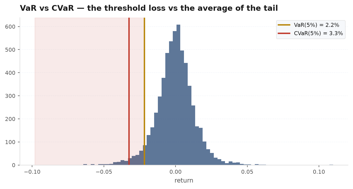
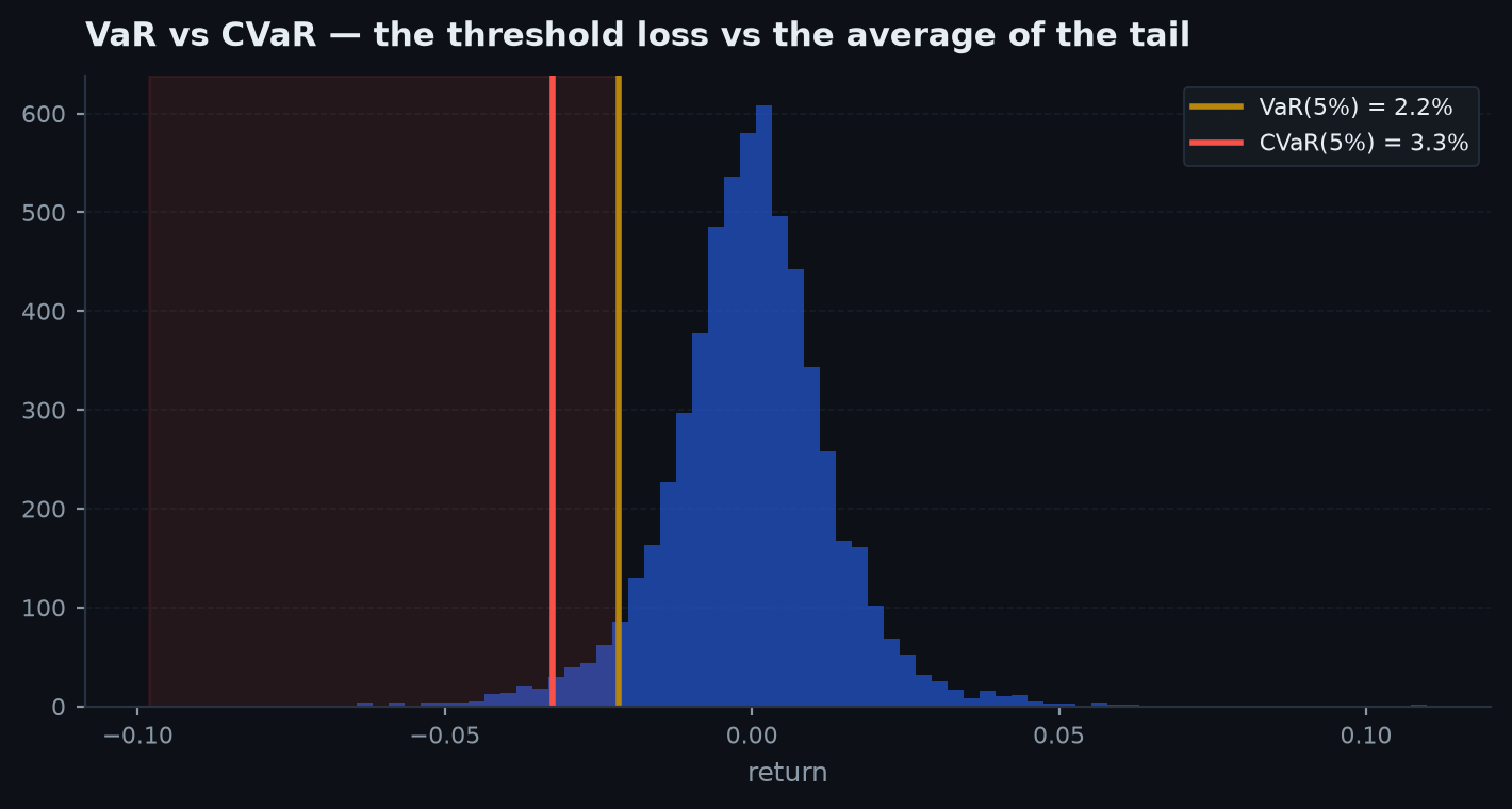
The payoff of POT is closed-form tail risk. With $n$ observations, $N_{u}$ exceedances of $u$ , and a fitted $(ξ, β)$ , the VaR at tail probability $α$ (e.g. 0.001) and its expected shortfall are:

VaR_{α} = u + \frac{β}{ξ} [(\frac{n α}{N _{u}})^{- ξ} - 1], ES_{α} = \frac{VaR _{α} + β - ξ u}{1 - ξ} .

→Derivation — VaR from the GPD survival function

For a loss $x > u$ , decompose the survival probability and substitute the GPD for the conditional excess:

P [X > x] = P [X > u] P [X > x ∣ X > u] \approx \frac{N _{u}}{n} (1 + ξ \frac{x - u}{β})^{- 1/ ξ} .

The VaR at level $α$ is the loss whose survival probability equals $α$ . Set the right-hand side to $α$ and solve for $x$ :

(1 + ξ \frac{x - u}{β})^{- 1/ ξ} = \frac{n α}{N _{u}} ⟹ x = u + \frac{β}{ξ} [(\frac{n α}{N _{u}})^{- ξ} - 1] . ■

For the ES, use the GPD’s mean-excess property: beyond any higher threshold $v > u$ the excess is again GPD with the same $ξ$ and scale $β + ξ (v - u)$ , so the expected excess over $VaR_{α}$ is $(β + ξ (VaR_{α} - u)) / (1 - ξ)$ . Adding the VaR back and simplifying gives the ES formula — finite only when $ξ < 1$ , another way the shape parameter polices which risk numbers exist.

A loss distribution with the VaR quantile marked and the expected-shortfall region shaded beyond it — VaR is a quantile of the loss distribution; ES is the average loss beyond it. Empirical estimates of both stop at the edge of the sample — EVT replaces the empirical tail with a fitted GPD so both can be evaluated past the worst observed day.

Worked scenario — extrapolating beyond the sample#

✦Scenario — 8 years of daily returns, and a 1-in-1000-day question

You hold $n = 2000$ daily equity returns (~8 years). The empirical 99% VaR is easy: the 20th worst day, say $3.1%$ . Now risk asks for the 99.9% VaR — a 1-in-1000-day loss. The empirical answer would be the 2nd worst observation: a sample statistic with catastrophic variance, and by construction it can never exceed your worst day. POT instead: threshold at the 95% quantile $u = 1.8%$ , so $N_{u} = 100$ exceedances; the fit gives $ξ^= 0.30$ , $β^= 0.9%$ . Plug into the formula with $α = 0.001$ :

VaR_{0.001} = 1.8 + \frac{0.9}{0.30} [(\frac{2000 \times 0.001}{100})^{- 0.30} - 1] = 1.8 + 3.0 [5 0^{0.30} - 1] \approx 1.8 + 3.0 \times 2.23 \approx 8.5%.

An $8.5%$ one-day loss — plausibly worse than anything in the sample — with $ES_{0.001} \approx (8.5 + 0.9 - 0.3 \times 1.8) /0.7 \approx 12.7%$ . A Gaussian fitted to the same data ( $σ \approx 1.2%$ ) would have said $3.09 \times 1.2 \approx 3.7%$ — less than half the EVT number. The Gaussian is not conservative in the tail; it is the most optimistic model you could legally write down.

evt_var.py

import edgekit as ek

r = prices.pct_change().dropna()             # daily returns, Series

# Fit the tail: losses beyond the 95% quantile, GPD via probability-weighted moments
fit = ek.risk.gpd_fit(-r, q=0.95)
print(fit)                                   # {"xi": ..., "beta": ..., "threshold": ..., "n_exceed": ...}

# EVT-based 99.9% VaR and expected shortfall (positive loss fractions)
var999, es999 = ek.risk.evt_var_es(r, alpha=0.001, q=0.95)
print(f"VaR 99.9%: {var999:.4f}, ES 99.9%: {es999:.4f}")

# Hill tail index for the honesty check — vary k, look for the plateau
for k in (25, 50, 100, 200):
    print(k, ek.risk.hill(-r, k=k))          # alpha = 1/xi; stable region = trustworthy

Assumptions versus reality#

EVT assumes	Reality	Consequence
i.i.d. observations	Volatility clusters — extremes arrive in bursts	Effective sample smaller; fit on residuals or accept wider error bands
Threshold u high enough for GPD limit	Finite samples force a bias-variance compromise	ξ estimates drift with u — report sensitivity, not one number
A stationary tail	Regimes change; microstructure and leverage evolve	Yesterday's ξ may not govern tomorrow's crash
Enough exceedances to fit (ξ, β)	The tail is, by definition, data-poor	Confidence intervals on 99.9% VaR are wide — honesty requires showing them

!EVT is disciplined extrapolation, not prophecy

The theorems earn EVT its extrapolation: if the tail is in a domain of attraction, its shape beyond the sample is pinned down by

ξ

. But the fit still rides on ~100 tail points, the i.i.d. assumption is wrong in the small (use GARCH-filtered residuals when it matters), and no theorem covers a mechanism change. Treat EVT-VaR the way this course treats every estimate — as a distribution, not a number — and pair it with the resampling machinery of the Monte-Carlo chapter.

Next: EVT measures the fat tail; the natural follow-up is what generates it. Jump processes and stochastic volatility are the two standard mechanisms that turn Gaussian noise into Fréchet-domain returns — and they explain the option-market smile along the way. Jumps & stochastic volatility.