Jumps & stochastic volatility

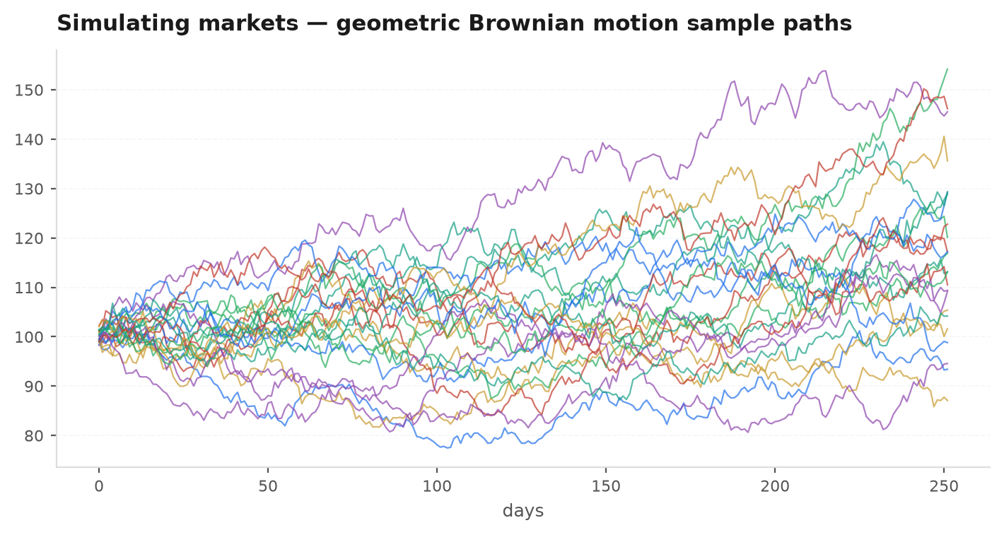
Geometric Brownian motion is the frictionless baseline of Part VI — and its failure table is a to-do list. This chapter crosses off the two biggest items. Adding a Poisson jump component (Merton) repairs the continuous-path lie; letting volatility be its own mean-reverting random process (Heston) repairs the constant- $σ$ lie. Together they generate the fat tails EVT measures and the implied-volatility smile the options market charges — the two symptoms turn out to share a mechanism.

✦Intuition — two ways to make a Gaussian world dangerous

Take pure GBM and ask: how do I make its returns look like real returns? Two levers. Jumps add rare, discontinuous shocks — the overnight gap, the surprise announcement — that no amount of diffusion can produce. Stochastic volatility keeps the noise Gaussian at each instant but makes its scale wander: returns become a mixture of normals with different variances, and mixtures of normals are fat-tailed. Markets use both levers. Jumps dominate the extreme short-horizon tail; wandering volatility produces the clustering you see in every squared-return ACF.

Where GBM breaks — the recap#

The assumptions table in Stochastic processeslisted four lies: Gaussian returns, constant volatility, continuous paths, independent increments. The first three are this chapter’s subject, and they are coupled — you cannot fix the Gaussian tail honestly without deciding why it is fat. The two canonical answers:

Discontinuity: prices jump. A hedger cannot trade through a jump, a stop cannot fill inside one, and a Gaussian diffusion assigns such moves essentially zero probability.
Non-stationary scale: the volatility that multiplies the Gaussian noise is itself random, persistent, and correlated with the price — high-vol episodes cluster and tend to follow drops.

Simulated geometric Brownian motion paths fanning out smoothly from a common starting price, with no gaps and a steady spread — The baseline being repaired: GBM paths are continuous everywhere and equally volatile everywhere. Compare with the Merton paths below — the difference is not cosmetic, it is where the tail risk lives.

Poisson processes and compound Poisson jumps#

The clock for rare events is the Poisson process $N_{t}$ : jumps arrive independently at rate $λ$ per unit time, so the number of jumps in $[0, t]$ is Poisson with mean $λ t$ , and inter-arrival times are exponential. Attach a random size to each jump — log-price moves $Y_{i} \sim N (μ_{J}, σ_{J}^{2})$ — and the running sum $\sum_{i = 1}^{N_{t}} Y_{i}$ is a compound Poisson process: flat between arrivals, discontinuous at them. This is the piece a diffusion cannot imitate.

Merton jump-diffusion#

Merton’s 1976 model welds compound Poisson jumps onto GBM:

\frac{d S}{S} = (μ - λκ) d t + σ d W + (e^{J} - 1) d N,

where $J \sim N (μ_{J}, σ_{J}^{2})$ is the jump in log-price, $d N$ is the Poisson increment, and the drift is compensated by $λκ$ with $κ = e^{μ_{J} + σ_{J}^{2} /2} - 1$ so the jumps do not smuggle in extra expected return. Between jumps the path is ordinary GBM; at a jump it gaps by the factor $e^{J}$ .

Simulated Merton jump-diffusion price paths showing smooth diffusive stretches interrupted by sudden discontinuous gaps, mostly downward — Merton jump-diffusion paths: GBM most of the time, punctuated by Poisson-timed gaps. With mu_J < 0 the gaps are mostly down — the overnight-crash risk that no continuous process, and no stop-loss order, can protect against.

→Derivation — the Merton price as a Poisson-weighted Black-Scholes series

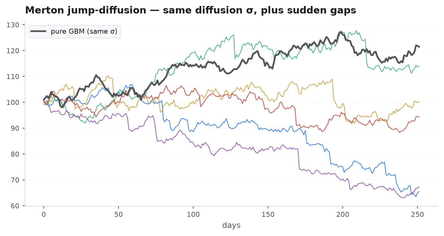
Condition on the number of jumps by expiry. Given $N_{T} = n$ , the log-price is Gaussian — a sum of the diffusion part and $n$ independent normal jumps — so the terminal price is log-normal with variance $σ_{n}^{2} T = σ^{2} T + n σ_{J}^{2}$ and a drift adjusted to $r_{n} = r - λκ + n (μ_{J} + σ_{J}^{2} /2) / T$ . Conditional on $n$ jumps, the option value is therefore an ordinary Black-Scholes price at those inputs. Average over the Poisson counts:

C_{Merton} = n = 0 \sum \infty \frac{e ^{- λ^{'} T} ( λ ^{'} T ) ^{n}}{n !} C_{BS} (S, K, T, r_{n}, σ_{n}), λ^{'} = λ (1 + κ) .

Why it matters: the terminal distribution is a log-normal mixture — Poisson weights on ever-wider Gaussians. Mixtures are fat-tailed, so out-of-the-money options are worth more than Black-Scholes at any single $σ$ — invert the price to an implied vol and you get a smile from a five-parameter model. The series converges fast; a few dozen terms suffice, which is what merton_price truncates at.

Heston stochastic volatility#

The second repair makes variance itself a state variable. Heston’s model is the SDE pair:

d S = μ S d t + v S d W^{(1)}, d v = κ (θ - v) d t + ξ v d W^{(2)}, corr (d W^{(1)}, d W^{(2)}) = ρ .

The variance $v_{t}$ mean-reverts toward the long-run level $θ$ at speed $κ$ , with vol-of-vol $ξ$ — the same square-root mean-reverting dynamic that a GARCH model expresses in discrete time. The load-bearing parameter is $ρ$ , and for equities it is strongly negative: price drops and volatility spikes are the same shock. That is the leverage effect, and it is what makes return distributions skewed, not just fat.

Fat tails: conditional on the variance path, returns are Gaussian — but variance wanders, so unconditional returns are a continuous mixture of normals. Excess kurtosis is automatic, growing with $ξ$ and the persistence $1/ κ$ .
Volatility clustering: mean reversion with persistence means high-variance states linger — the vol-clustering stylised fact falls out of the $d v$ equation directly.
Skew: with $ρ < 0$ , downside moves happen in high-variance states and get amplified; upside moves happen in calm states. The left tail fattens more than the right.

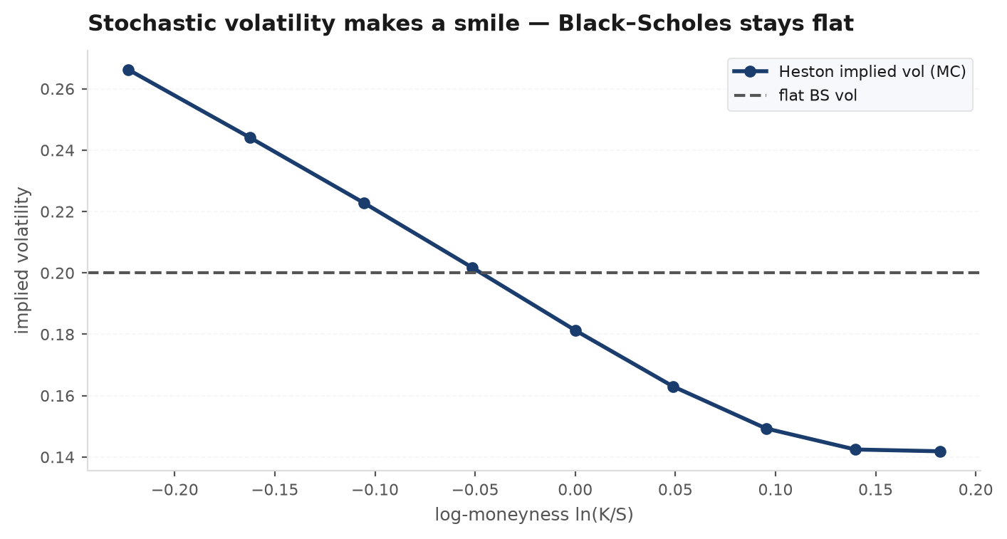
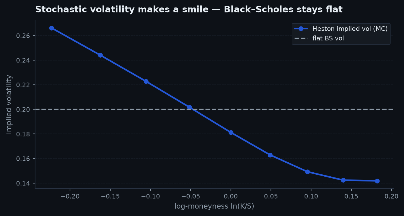
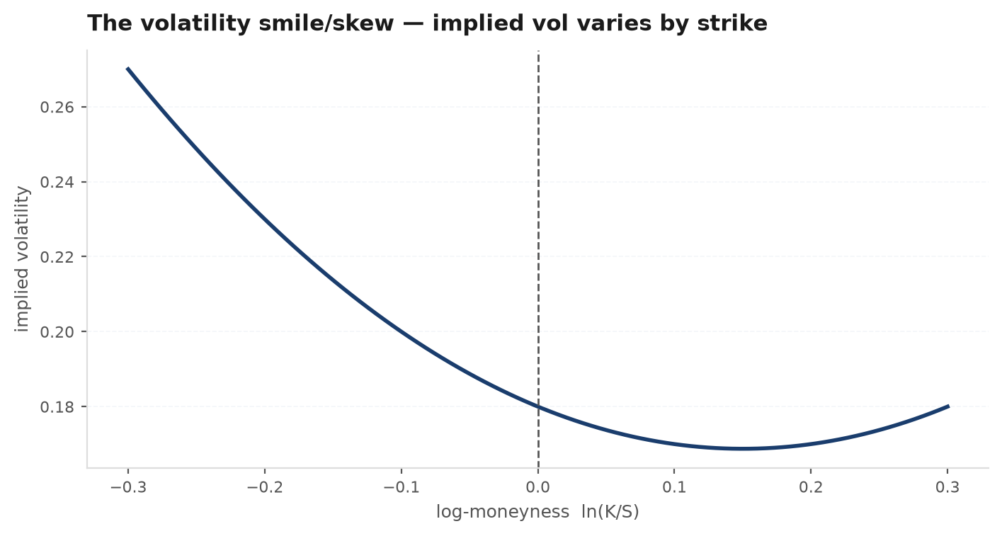
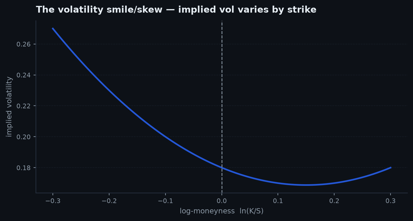
Implied volatility versus strike generated by a Heston model with negative rho, showing a downward-sloping skew with a smile floor — The implied-vol curve a Heston model generates. Vol-of-vol bends both wings up (a smile); negative rho tilts it into a skew — low strikes trade at higher implied vol because crashes and vol spikes arrive together. The market's observed surface has exactly this shape.

Read against the option market’s observed volatility smile: Black-Scholes at constant $σ$ predicts a flat implied-vol line. Jumps bend the short-dated wings up; stochastic volatility with $ρ < 0$ tilts the whole curve into the persistent equity skew. The smile is not an anomaly — it is the market pricing the very deviations from GBM this chapter models.

Observed implied volatility smile across strikes compared to the flat line Black-Scholes would predict — What the market actually charges: implied vol versus strike is a skewed smile, not the flat line of constant-sigma GBM. Merton jumps and Heston dynamics are the two standard mechanisms that reproduce it.

Variance as a mean-reverting process#

Step back from option pricing and the $d v$ equation is interesting on its own. It says variance is a forecastable time series: displaced from $θ$ , it decays back at rate $κ$ , so today’s variance predicts tomorrow’s with a half-life of $ln 2/ κ$ . This is the continuous-time statement of the single most robust stylised fact in finance — volatility is persistent and mean-reverting — and it is the same structure a GARCH(1,1) recursion expresses bar by bar, where $α + β$ plays the role of persistence and $ω / (1 - α - β)$ the role of $θ$ . Everything the ARIMA & GARCH chapter does with conditional variance — forecasting it, scaling positions by it, filtering returns to near-i.i.d. residuals — is the discrete shadow of the Heston variance equation.

→Simulating Heston honestly — full truncation

The variance SDE has no exact discretisation, and a naive Euler step can drive

v

negative, at which point

v

is undefined. The full-truncation Euler scheme — use

max (v, 0)

inside both the drift and the diffusion, keep the raw

v

in the state — is the standard low-bias fix, and it is what heston_paths implements. Related fine print: the Feller condition

2 κ θ \geq ξ^{2}

keeps the continuous process strictly positive, but realistic equity calibrations routinely violate it — the variance path genuinely visits zero, and the simulation scheme has to survive that rather than assume it away.

Worked scenario — same total σ, with and without jumps#

✦Scenario — where did the 1% days go?

Build two return processes with the same annualised volatility of $20%$ (daily $σ_{d} \approx 1.26%$ ). Process A: pure GBM. Process B: Merton with $λ = 5$ jumps/year, $μ_{J} = - 2%$ , $σ_{J} = 3%$ , and the diffusive $σ$ reduced so total variance matches: $σ_{diff}^{2} = 0.04 - λ (μ_{J}^{2} + σ_{J}^{2}) = 0.04 - 5 \times 0.0013 = 0.0335$ , i.e. $σ_{diff} \approx 18.3%$ . Same second moment — a variance scan cannot tell them apart. Now look at the tails. For GBM a $- 5%$ day is a $4 σ$ event: probability $\approx 3 \times 1 0^{- 5}$ per day, once per ~130 years. For the jump process, a single jump lands below $- 5%$ with probability $Φ ((- 5 + 2) /3) = Φ (- 1) \approx 16%$ , and jumps arrive 5 times a year — so roughly 0.8 such days per year, about a hundred times the Gaussian rate. Identical headline vol, utterly different 99.9% quantiles: this is the mechanism behind the EVT chapter’s $ξ > 0$ , and why sizing off $σ$ alone is a category error.

jump_tails.py

import numpy as np
import edgekit as ek

# Same total variance, with and without jumps
S_gbm = ek.sim.gbm_paths(100.0, 0.05, 0.20, t=1.0, steps=252, n_paths=20_000)
S_jump = ek.sim.merton_paths(100.0, 0.05, 0.183, lam=5.0, jump_mu=-0.02,
                             jump_sigma=0.03, t=1.0, steps=252, n_paths=20_000)

r_gbm = np.diff(np.log(S_gbm), axis=1).ravel()
r_jump = np.diff(np.log(S_jump), axis=1).ravel()
for p in (0.01, 0.001):                       # daily tail quantiles
    print(p, np.quantile(r_gbm, p), np.quantile(r_jump, p))

# Heston: joint price and variance paths (full-truncation Euler)
S, V = ek.sim.heston_paths(100.0, 0.05, v0=0.04, kappa=2.0, theta=0.04,
                           xi=0.6, rho=-0.7, t=1.0, steps=252, n_paths=10_000)

# The smile a jump model implies: invert Merton prices strike by strike
c = ek.options.merton_price(100.0, 90.0, 0.25, 0.02, 0.183,
                            lam=5.0, jump_mu=-0.02, jump_sigma=0.03, kind="put")

Assumptions versus reality#

Model	Repairs	Still assumes	Consequence
GBM	—	Thin tails, constant σ, continuity	The baseline null; wrong in every tail
Merton	Gaps, short-dated smile, kurtosis	Constant σ between jumps; jump params stable	No vol clustering; crash rate itself drifts
Heston	Clustering, skew, term structure of vol	Continuous paths; one vol factor	Underprices overnight gaps and short-dated wings
Both (Bates)	Tails and clustering together	Parameters constant across regimes	Calibration drifts — re-fit and monitor

!More parameters, more places to be fooled

Merton adds three parameters, Heston five, and both can fit yesterday’s surface beautifully while mispricing tomorrow’s. The estimation problem is real: jumps are rare (so

λ, μ_{J}, σ_{J}

have wide error bars) and vol-of-vol trades off against correlation in the fit. Use these models the way this course uses every model — as scenario generators for stress, not oracles. Simulating a strategy on Merton and Heston paths with matched overall volatility, as above, is one of the cheapest robustness checks in the simulation toolkit.

Next: jumps and stochastic vol describe randomness in the time domain. There is a second lens — decompose the series into frequencies and ask which cycles are real. It is powerful, and it is one of the easiest ways in quantitative finance to fool yourself. Fourier analysis & cycles.