Fourier analysis & cycles

Any series can be rewritten as a sum of sinusoids, and the periodogram tells you how much variance lives at each frequency. That makes Fourier analysis a genuine detector of seasonality — intraday volume rhythms, day-of-week effects — and simultaneously one of the great engines of self-deception in trading, because pure noise always produces impressive-looking peaks. This chapter builds the periodogram from the DFT, explains why it must be smoothed to estimate a spectrum, and draws the line between a cycle that survives a permutation test and a cycle that is just the noise you went looking for.

✦Intuition — a prism for time series

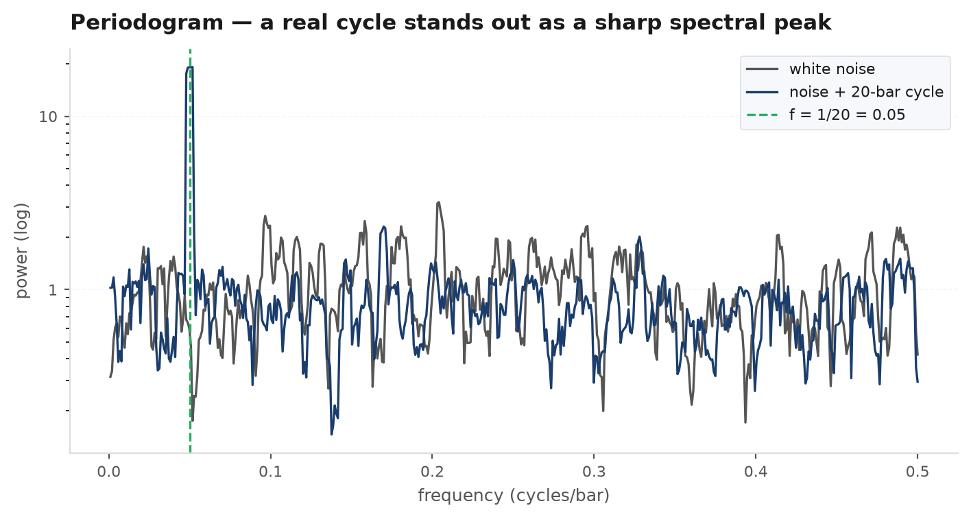
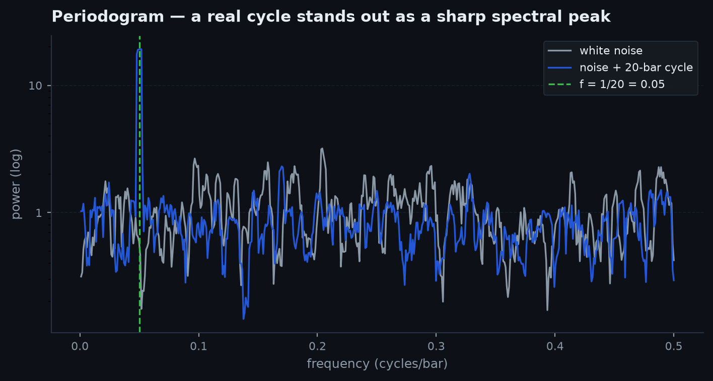
A prism splits light into its component colours and shows you the energy at each wavelength. The discrete Fourier transform does the same for a time series: it re-expresses the data as a sum of sines and cosines and reports the amplitude at each frequency. A genuine cycle — something in the world that repeats, like the opening and closing rush of trading volume — concentrates variance at its frequency and shows up as a sharp, reproducible spectral line. The trap is that white noise does not produce a flat-looking periodogram on any finite sample: it produces a jagged forest of spurious peaks. The skill is not finding peaks — anyone can find peaks — it is knowing which ones would survive on data that has no cycles at all.

The periodogram, from the DFT#

Take a demeaned series $x_{0}, \dots, x_{n - 1}$ sampled once per bar. Its discrete Fourier transform evaluates the correlation of the data with a complex sinusoid at each Fourier frequency $f_{j} = j / n$ , in units of cycles per bar:

X (f_{j}) = t = 0 \sum n - 1 x_{t} e^{- 2 π i f_{j} t}, j = 0, 1, \dots, ⌊ n /2 ⌋ .

The periodogram is the squared magnitude, normalised by the sample size:

I (f_{j}) = \frac{1}{n} X (f_{j})^{2} .

Read it as a variance budget: summing $I (f_{j})$ across frequencies recovers (up to convention) the sample variance, so each ordinate is the share of variance explained by a sinusoid at that frequency. A frequency of $f = 0.05$ cycles/bar means a period of $1/ f = 20$ bars; the highest resolvable frequency is the Nyquist limit $f = 0.5$ — one full cycle every two bars. For real-valued data the negative frequencies are redundant, which is why periodogram uses the real FFT and returns only $[0, 0.5]$ .

A raw periodogram of a return series: a jagged spiky curve across frequency, with one candidate peak highlighted among many spurious ones — A raw periodogram. The jaggedness is not information — it is the estimator's own variance. Every finite sample of pure noise produces spikes like these; the tallest one is always somewhere. The question is never whether a peak exists but whether it survives smoothing and a permutation null.

Spectral density — and why raw periodograms lie#

The object the periodogram is trying to estimate is the spectral density $S (f)$ — the Fourier transform of the autocovariance function, describing how the process distributes variance over frequency in expectation. Two facts anchor all interpretation:

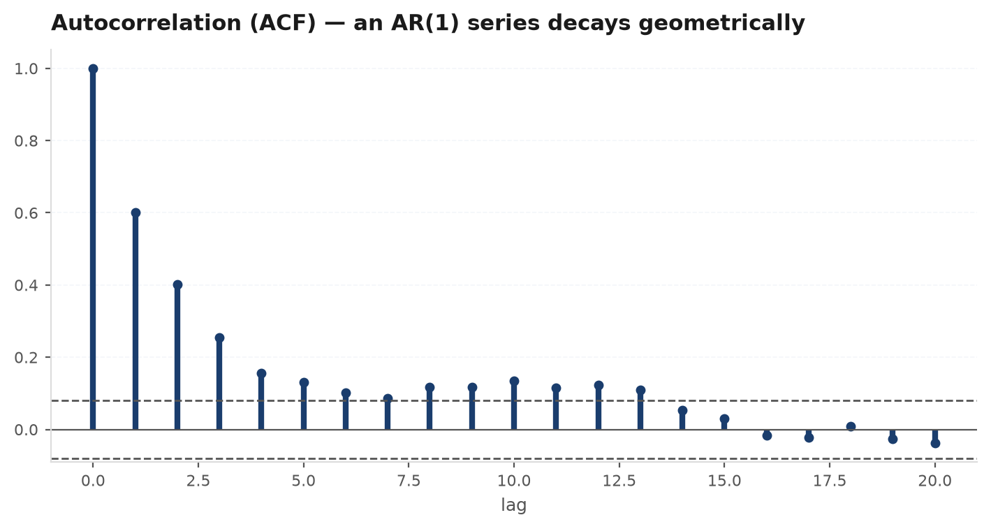
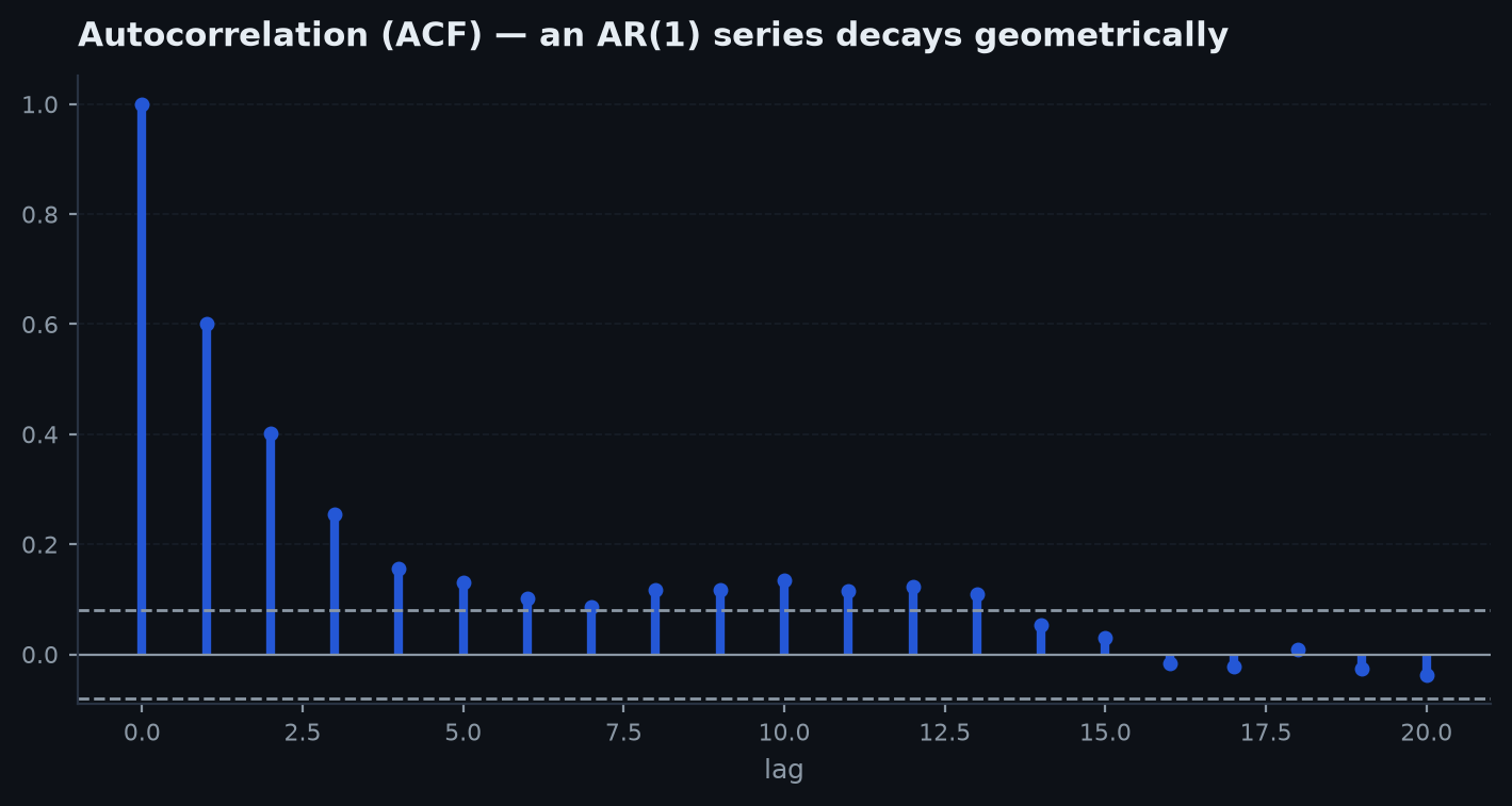
White noise is flat: for i.i.d. noise with variance $σ^{2}$ , the spectral density is constant, $S (f) = σ^{2}$ for all $f$ — every frequency carries equal variance, which is precisely why it is called white. A flat spectrum is the frequency-domain twin of the zero-autocorrelation null you test with an ACF plot.
The raw periodogram is inconsistent: at any fixed frequency, $I (f)$ is approximately distributed as $S (f) χ_{2}^{2} /2$ — an exponential-type variable whose standard deviation equals its mean — and this does not improve with more data. More observations buy you more frequencies, not less noise per frequency. The estimator’s variance never shrinks.

An autocorrelation plot of returns with bars inside the significance band at every lag, the time-domain counterpart of a flat spectrum — The time-domain twin: an ACF with no significant lags corresponds to a flat spectral density. The periodogram and the ACF are Fourier transforms of each other — a cycle at period p in one is a damped ripple at lag p in the other, and both inherit the same estimation noise.

→Derivation sketch — why more data doesn't help, and what does

At frequency $f_{j}$ the DFT is a sum of $n$ terms; under mild conditions its real and imaginary parts are asymptotically independent normals with variance $n S (f_{j}) /2$ each. The periodogram divides the squared magnitude by $n$ , so

I (f_{j}) \approx \frac{S ( f _{j} )}{2} (Z_{1}^{2} + Z_{2}^{2}) = S (f_{j}) \frac{χ _{2}^{2}}{2},

a two-degree-of-freedom quantity regardless of $n$ — the $n$ s cancel. Doubling the sample halves the frequency spacing but leaves each ordinate just as noisy. The repair is to trade resolution for stability: average the periodogram over $m$ neighbouring frequencies (a Daniell window), which sums approximately independent $χ_{2}^{2}$ variables into a $χ_{2 m}^{2}$ — relative standard error $1/ m$ . That smoothing is exactly what spectral_density does, and it is the difference between an estimator and a random-number generator.

Prepare the series first — the red-spectrum trap#

One preprocessing mistake produces more fake cycles than any other: transforming the wrong series. A random walk — prices under the martingale null — has a spectrum proportional to $1/ f^{2}$ : enormous power at low frequencies, decaying smoothly. Feed raw prices to the periodogram and you get a mountain range at the left edge that looks like a majestic long-period cycle and is nothing but accumulated noise. The same applies to any trending or slowly wandering series.

Analyse returns (or differences), not levels. Differencing is a high-pass filter that flattens the random-walk spectrum back to white — the correct null for the search.
Demean always (a nonzero mean is a spike at $f = 0$ that leaks into neighbouring frequencies), which periodogram does for you.
Mind the sampling rate. Frequencies are in cycles per bar: a cycle faster than two bars is aliased — folded back onto a lower frequency — and invisible at your resolution.

Real cycles versus noise peaks#

What does a genuine cycle look like? Three signatures separate it from a noise spike:

It survives smoothing. A true spectral line keeps its prominence when the periodogram is Daniell-smoothed; a noise spike is averaged away with its neighbours.
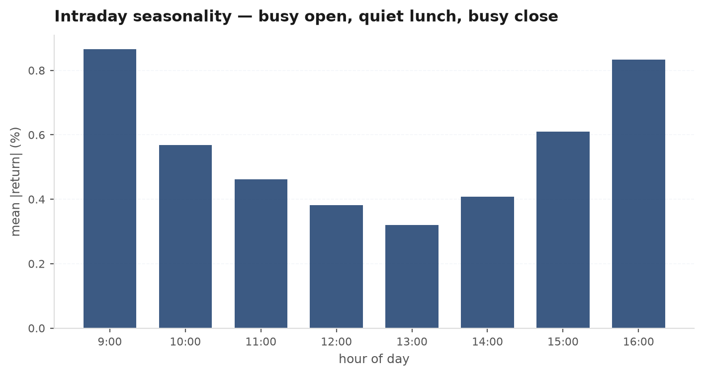
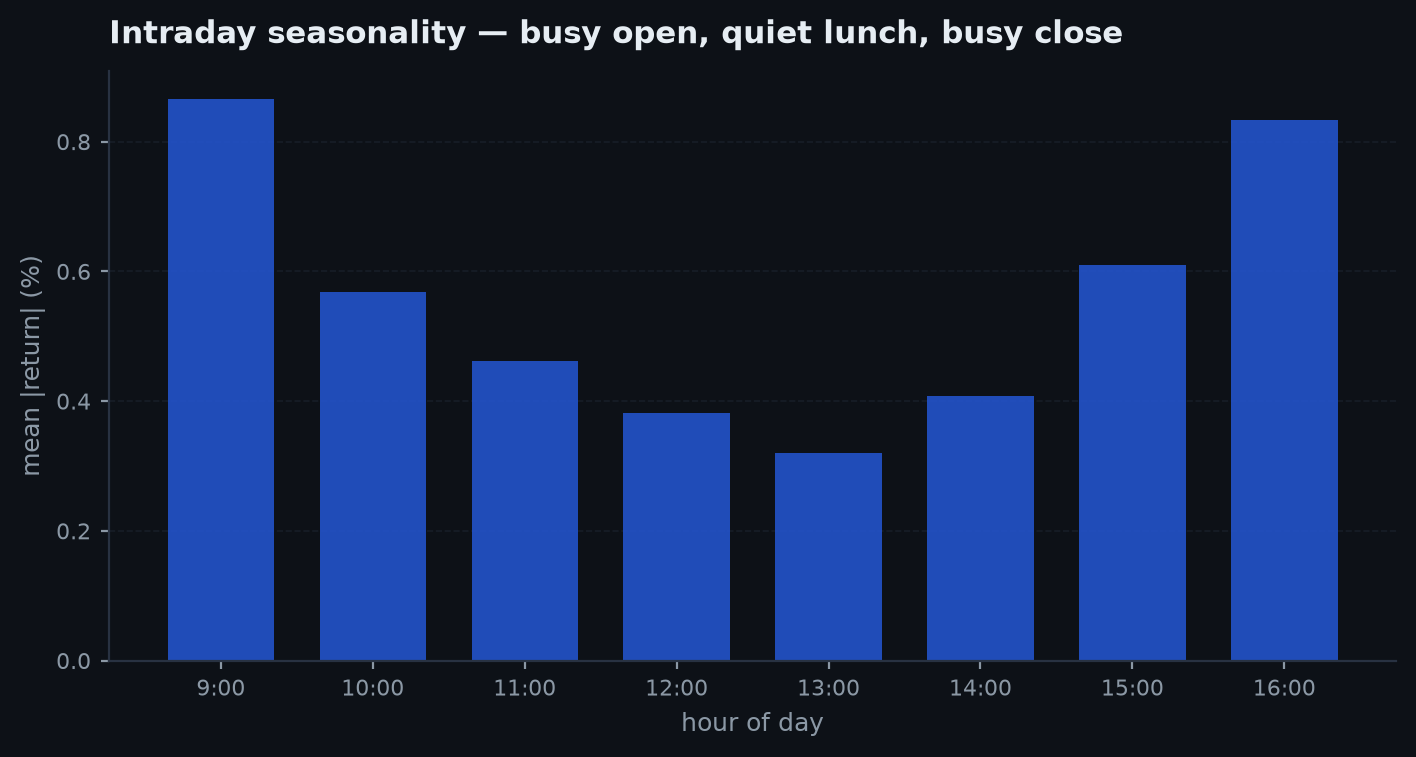
It has a mechanism and a stable frequency. Intraday volume peaks at the open and close because auctions, hedging flows, and order deadlines happen at clock times. The cycle sits at exactly one bar-count per session, every session, in every subsample.
It replicates out of sample. Split the data: a real cycle appears at the same frequency in both halves. A noise peak relocates.

Smoothed spectrum of intraday volume showing a dominant sharp peak at the session frequency and its harmonic, towering above a flat background — A real cycle: the smoothed spectrum of intraday volume. The session-frequency peak (and its harmonic) stands far above the background, survives smoothing, and reappears in every subsample — because it is caused by the clock, not discovered in the noise.

!The multiple-comparisons trap of cycle-hunting

A periodogram on

n = 2000

bars hands you a thousand frequencies — a thousand simultaneous hypothesis tests. Under the white-noise null the maximum ordinate is roughly

S \cdot ln (n /2)

, several times the average level, so the tallest peak in pure noise always looks “significant” against a naive single-frequency threshold. Scanning the spectrum for the best-looking cycle and then testing that same cycle on the same data is the frequency-domain edition of the selection bias in Why backtests lie: the search itself manufactures the significance. Fisher’s g-test corrects for the scan analytically; the permutation test below does it by brute force and generalises to any statistic.

The honest test: a permutation null#

The cleanest defence needs no distributional assumptions. Shuffling the observations in time destroys any cyclical structure while exactly preserving the marginal distribution — fat tails and all. So: compute your statistic (say, the maximum periodogram ordinate, or the power at the claimed frequency) on the real data, then on many shuffles, and ask how often the shuffles beat reality.

p = \frac{1 + # { shuffles with T _{shuffle} \geq T _{real} }}{1 + N _{shuffles}} .

Using the maximum ordinate as the statistic bakes the multiple-comparisons correction into the null: each shuffle also gets to show off its own tallest peak, so the comparison is search-against-search — the same logic as the Monte-Carlo permutation tests that guard the gauntlet.

Worked scenario — a real cycle and a fake one#

✦Scenario — intraday volume vs the “35-bar price cycle”

Two claims on 5-minute data, 78 bars per session, $n = 3900$ bars (50 sessions). Claim 1: volume is seasonal within the day. The smoothed spectrum of volume shows a peak at $f = 1/78 \approx 0.0128$ cycles/bar rising ~40× above the background, with a clear harmonic at $2/78$ . Permutation test on the max ordinate: none of 1000 shuffles comes close — $p \approx 0.001$ . Both halves of the sample show the peak at the identical frequency. Real, strong, mechanistic — the U-shaped volume curve every intraday trader knows. Claim 2: returns have a 35-bar cycle (a peak spotted at $f \approx 0.0286$ ). The raw ordinate is 6× the average level — impressive until you note the scan covered 1950 frequencies, and the expected maximum under white noise is $ln (1950) \approx 7.6$ times the mean. The permutation null agrees: 62% of shuffles produce a tallest peak at least this large, $p \approx 0.62$ . Smoothing flattens it; the second half of the sample puts its best peak near 23 bars instead. The 35-bar cycle is the noise’s tallest tree, photographed and named.

cycle_hunt.py

import numpy as np
import edgekit as ek

# Raw periodogram: frequencies in cycles/bar, power per frequency
freq, power = ek.timeseries.periodogram(volume)          # demeaned, rfft-based
print(freq[np.argmax(power)], 1 / freq[np.argmax(power)])  # peak freq and period in bars

# Consistent estimate: Daniell-smoothed spectral density
freq_s, dens = ek.timeseries.spectral_density(volume, n_smooth=7)

# Permutation null for the MAX ordinate (search-vs-search, multiplicity-aware)
rng = np.random.default_rng(11)
t_real = power.max()
t_null = np.empty(1000)
for i in range(1000):
    _, p_sh = ek.timeseries.periodogram(np.asarray(volume)[rng.permutation(len(volume))])
    t_null[i] = p_sh.max()
p_value = (1 + (t_null >= t_real).sum()) / (1 + len(t_null))
print(f"max-peak permutation p = {p_value:.3f}")

Assumptions versus reality#

Spectral analysis assumes	Reality	Consequence
Stationarity over the sample	Regimes, trends, drifting volatility	Power smears across frequencies; detrend and difference first
Fixed, persistent cycle frequency	Market rhythms drift with the calendar and microstructure	Yesterday's peak frequency mislocates tomorrow's
One test at one frequency	You scanned every frequency for the best peak	Naive p-values are fiction — test the max, or use Fisher's g
A peak implies a tradeable signal	Volume/vol seasonality is real; price cycles rarely survive costs	Spectral edges must still run the full gauntlet

The honest summary: Fourier methods are excellent at confirming structure you have a mechanism for — seasonality in volume, volatility, spreads — and dangerous as a discovery tool for price cycles, because the estimator is noisy, the search is wide, and the null is never flat-looking. Treat the periodogram like a backtest: it only means something relative to what noise alone would have shown you.

Next: this closes Part IX — dependence, extremes, jumps, and cycles. The next part changes altitude: from the behaviour of prices to the cross-section of expected returns — factors, premia, and how to test whether a characteristic is actually paid. Factor investing.