Regression & factor models

Every strategy’s return can be split into a part explained by things you did not choose — the market, a sector, a style — and a residual that is genuinely yours. Regression is the tool that does the splitting, and the CAPM is the simplest useful example: it separates skill (alpha) from riding the market (beta). This chapter derives ordinary least squares from first principles, shows where its standard errors and t-stats come from, and wires the theory straight into ek.factors.

✦Intuition — why a trader cares before any algebra

Your crypto strategy returned $+ 40%$ last year. Impressive — until you notice Bitcoin itself was up $+ 70%$ . So how much of that $40%$ was you, and how much was just being in the room while the market rose? Regression answers exactly that. It draws the best straight line through “my return” versus “the market’s return,” and the line has two numbers: a slope (how much you move when the market moves — the part you did not earn) and a height where the market return is zero (what you made when the market did nothing — the part that might be skill). Splitting those two apart, and asking whether the second is real or a fluke, is the whole game. Everything below is the machinery that draws that line honestly.

The linear model#

We posit that a response $y$ (say, a strategy’s daily returns) is a linear combination of $k$ explanatory variables, plus noise. Stacking $n$ observations into a vector $y \in R^{n}$ and the regressors into a design matrix $X \in R^{n \times k}$ (one column per variable, usually including a column of ones for the intercept):

y = X β + ε, E [ε] = 0, Var (ε) = σ^{2} I .

The unknown coefficient vector $β \in R^{k}$ is what we want to estimate, and $ε$ is the part of $y$ the regressors cannot explain. The assumptions on the right — zero-mean, constant-variance, uncorrelated errors — are what make least squares the best linear unbiased estimator (the Gauss-Markov theorem); we will flag where financial data violates them.

Ordinary least squares — the normal equations#

OLS chooses the $β$ that minimises the sum of squared residuals (SSR) — the total squared vertical distance between the data and the fitted line:

S (β) = t = 1 \sum n (y_{t} - x_{t}^{⊤} β)^{2} = (y - X β)^{⊤} (y - X β) .

✦Derivation — minimise the SSR to get β = (XᵀX)⁻¹Xᵀy

Expand the objective, using $(X β)^{⊤} y = y^{⊤} X β$ (both scalars, equal to their own transpose):

S (β) = y^{⊤} y - 2 β^{⊤} X^{⊤} y + β^{⊤} X^{⊤} X β .

This is a convex quadratic in $β$ (the Hessian $2 X^{⊤} X$ is PSD), so the unique minimum is where the gradient vanishes. Differentiating with the matrix-calculus rules $\nabla_{β} (β^{⊤} a) = a$ and $\nabla_{β} (β^{⊤} A β) = 2 A β$ :

\nabla_{β} S = - 2 X^{⊤} y + 2 X^{⊤} X β =! 0 ⟹ X^{⊤} X β = X^{⊤} y .

Those are the normal equations. When $X^{⊤} X$ is invertible (the regressors are not collinear), solve for the estimator:

β^= (X^{⊤} X)^{- 1} X^{⊤} y .

Geometric reading. The fitted values $y^= X β^= X (X^{⊤} X)^{- 1} X^{⊤} y = H y$ are the orthogonal projection of $y$ onto the column space of $X$ ; the normal equations are just the statement that the residual $ε^= y - y^$ is perpendicular to every regressor, $X^{⊤} ε^= 0$ . Least squares is the closest point in the span of your explanatory variables — nothing more.

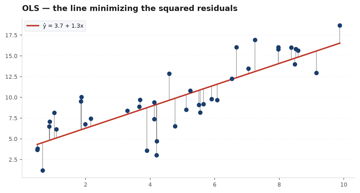
A scatter of points with the least-squares regression line through them and vertical residual segments from each point to the line — Ordinary least squares in one picture. The line is the beta that minimises the summed squares of the vertical residual segments; the normal equations are exactly the condition that no other line makes those segments jointly shorter. The fit is the orthogonal projection of the data onto the regressors.

edgekit computes exactly this in ek.factors.ols, using numpy.linalg.lstsq (which solves the normal equations stably via a matrix factorisation rather than forming $(X^{⊤} X)^{- 1}$ naively). Set add_const=True to prepend the intercept column automatically.

ols.py

import edgekit as ek

res = ek.factors.ols(y, X, add_const=True)   # X without a constant column
res["beta"]     # coefficients, intercept first
res["se"]       # standard errors
res["tstat"]    # beta / se
res["r2"]       # coefficient of determination
res["resid"]    # y - fitted (the unexplained part)

Goodness of fit: R²#

How much of the variation in $y$ did the model capture? The residual is orthogonal to the fit, so the total variation splits cleanly (Pythagoras in $n$ dimensions) into explained plus unexplained:

SST t \sum (y_{t} - y ˉ)^{2} = SSE t \sum (y^_{t} - y ˉ)^{2} + SSR t \sum (y_{t} - y^_{t})^{2} .

The coefficient of determination is the explained fraction:

R^{2} = 1 - \frac{SSR}{SST} = \frac{SSE}{SST} \in [0, 1] .

An $R^{2}$ of 0.7 in a CAPM regression means 70% of the strategy’s return variance is just the market moving. Adding regressors can only raise $R^{2}$ (a projection onto a bigger space can only get closer), which is why edgekit also reports adj_r2 — it penalises extra columns and can fall when a regressor adds nothing.

!High R² is not high skill

A strategy with

R^{2} = 0.9

against the market has almost no independent signal — it is the market with a bit of noise. For finding alpha you want a low

R^{2}

on the systematic factors and a significant intercept. Fit quality and edge are different questions.

Standard errors and t-stats#

A point estimate $β^$ is useless without a sense of its uncertainty. Under the model assumptions the estimator’s sampling covariance follows from $β^= (X^{⊤} X)^{- 1} X^{⊤} y$ being a linear function of the random $y$ :

Var (β^) = σ^{2} (X^{⊤} X)^{- 1}, σ^^{2} = \frac{SSR}{n - k} .

The standard error of coefficient $j$ is the square root of the $j$ -th diagonal entry, and the t-statistic asks how many standard errors the estimate sits away from zero:

se (β^_{j}) = σ^^{2} [(X^{⊤} X)^{- 1}]_{j j}, t_{j} = \frac{β ^ _{j}}{se ( β ^ _{j} )} .

A $∣ t ∣ ≳ 2$ is the rough “significant at 5%” bar: the coefficient is unlikely to be that far from zero by chance. edgekit returns se and tstat from ols using the unbiased $n - k$ denominator.

!Return data breaks the plain-OLS standard errors

The formula

σ^{2} (X^{⊤} X)^{- 1}

assumes errors are uncorrelated and equal-variance. Financial returns are neither — volatility clusters (heteroskedasticity) and overlapping holds induce autocorrelation, which makes plain SEs too small and t-stats too optimistic. edgekit provides ek.factors.newey_west_se (a HAC sandwich estimator) for exactly this; treat a

t = 2.1

on serially-correlated returns with suspicion.

The CAPM: alpha vs beta#

The Capital Asset Pricing Model is a one-regressor OLS with a famous interpretation. Regress an asset’s excess return (over the risk-free rate $r_{f}$ ) on the market’s excess return:

r_{i} - r_{f} = α + β (r_{m} - r_{f}) + ε .

The two coefficients answer two different questions:

Beta ( $β$ ) is market exposure. The slope is $β = Cov (r_{i}, r_{m}) / Var (r_{m})$ — how much the asset moves per unit of market move. A trend-follower that is secretly just long the index shows $β \approx 1$ . Beta is the return you could have earned with an index fund; it is not skill.
Alpha ( $α$ ) is skill. The intercept is the average excess return left over after stripping out the market. A positive, statistically significant $α$ is the evidence that a strategy adds something the market did not give away for free.

The test of skill is therefore a t-test on the intercept. edgekit’s ek.factors.capm returns alpha, beta, the t-stat on alpha (alpha_t), the t-stat on beta (beta_t), the fit (r2), and an annualised intercept (alpha_annual) for a readable number. The bar you want to clear is a positive alpha with $∣ alpha_t ∣ ≳ 2$ .

capm.py

import edgekit as ek

cm = ek.factors.capm(asset_returns, market_returns, rf=0.0,
                     periods_per_year=252)
cm["beta"]          # market exposure (1.0 = moves with the index)
cm["alpha"]         # per-period skill, net of the market
cm["alpha_t"]       # t-stat on alpha: is the skill real?  (|t| > 2)
cm["alpha_annual"]  # alpha scaled to a yearly number
cm["r2"]            # fraction of variance the market explains

✦Scenario — splitting a crypto strategy's return into alpha and beta

Regress a trend strategy’s monthly excessreturns on BTC’s monthly excess returns over 36 months. Suppose OLS hands back $β = 0.55$ , $α = 0.8% /month$ with $se (α) = 0.4%$ , and $R^{2} = 0.45$ . Over that window BTC’s excess return averaged $2.5% /month$ . Decompose the strategy’s average month:

strategy 2.175% = α, skill 0.8% + β (r_{m} - r_{f}) = 1.375%, market ride 0.55 \times 2.5% .

Annualised, that is $0.8% \times 12 \approx 9.6%$ of alpha versus $1.375% \times 12 \approx 16.5%$ you could have earned with $0.55$ units of a BTC index fund. More than half the “edge” was beta. Now the honesty check: $t_{α} = 0.8/0.4 = 2.0$ — it just clears the bar, but only just. And because monthly returns overlap and cluster, the plain SE is optimistic; run ek.factors.newey_west_se and a HAC correction of even $25%$ pushes $t_{α}$ to $1.6$ — no longer significant. The point-estimate looked like skill; the inference says “plausibly, but unproven.”

→This is the honest version of is_it_beta

The gauntlet’s ek.validation.is_it_beta gives a quick annualised intercept with np.polyfit. ek.factors.capm is the inference-carrying version: it hands you the t-stat, so you can distinguish “alpha looks positive” from “alpha is statistically distinguishable from zero.” A positive point-estimate with

alpha_t = 0.6

is not skill — it is noise. See Alpha vs beta for the trading interpretation.

The security market line#

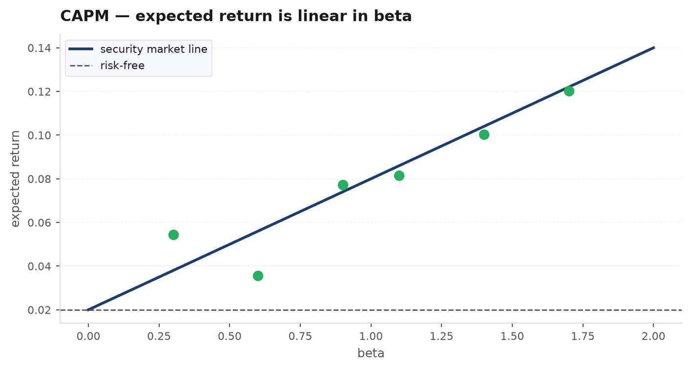
CAPM makes an equilibrium prediction: across assets, expected excess return should be a straight line in beta — the security market line (SML), $E [r_{i} - r_{f}] = β_{i} (E [r_{m}] - r_{f})$ . An asset with no skill sits on the line; its whole return is compensation for the market risk it carries. An asset with genuine alpha sits above it — the vertical gap is the alpha.

Multi-factor models#

A single market factor rarely explains everything. The Fama-French insight was that a couple more systematic factors — a size spread (small minus big, SMB) and a value spread (high minus low book-to-market, HML) — capture return variation the market misses. The regression just grows more columns:

r_{i} - r_{f} = α + β_{mkt} (r_{m} - r_{f}) + β_{smb} SMB + β_{hml} HML + ε .

Same normal equations, wider $X$ . Now each $β$ is a loading — how much of the strategy’s return is explained by each known factor — and the intercept $α$ is the return left after controlling for allof them. This is the harder, fairer bar: a “market-neutral” strategy can have $β_{mkt} \approx 0$ yet be quietly loaded on value, and its apparent alpha vanishes once HML is in the regression.

edgekit’s ek.factors.factor_exposures runs this multivariate OLS. Pass the asset returns and a DataFrame of factor returns; it returns betas and tstats as dicts keyed by your factor column names, plus alpha, alpha_t, and r2.

factors.py

import edgekit as ek
import pandas as pd

factors = pd.DataFrame({"mkt": mkt_ret, "smb": smb_ret, "hml": hml_ret})
fx = ek.factors.factor_exposures(asset_returns, factors)

fx["betas"]     # {"mkt": 0.08, "smb": 0.41, "hml": -0.22}  loadings by name
fx["tstats"]    # {"mkt": 0.7, "smb": 3.9, "hml": -2.1}     significance by name
fx["alpha"]     # intercept AFTER controlling for every factor
fx["alpha_t"]   # is the leftover alpha real?
fx["r2"]        # variance spanned by the factors together

✦Scenario — a 'market-neutral' alpha that was really a value tilt

A long/short equity book reports a CAPM fit of $β_{mkt} = 0.05$ (looks genuinely neutral) and $α = 6% /yr$ with $t_{α} = 2.4$ — apparently real skill uncorrelated to the index. Add the Fama-French value factor and re-run:

r - r_{f} = α + 0.05 (r_{m} - r_{f}) + 0.45 HML + ε, t_{hml} = 3.9.

The HML loading is $0.45$ with $t = 3.9$ — the book is quietly long cheap stocks and short expensive ones. With that captured, the intercept collapses to $α = 1.5% /yr$ at $t_{α} = 0.6$ . The “alpha” was never neutral skill; it was compensation for bearing value risk, a factor you can rent for a few basis points. Market-neutral in the $β_{mkt}$ sense is not factor-neutral. This is why the fair bar is a significant intercept after all the obvious factors are in the regression, not just after the market.

Quantity	Formula	Reads as	edgekit key
OLS estimator	$(X^{⊤} X)^{- 1} X^{⊤} y$	Best-fit coefficients	beta
Standard error	$σ^^{2} [(X^{⊤} X)^{- 1}]_{j j}$	Estimate uncertainty	se
t-statistic	$β^_{j} / se$	Significant if \|t\| ≳ 2	tstat / alpha_t
Fit	$1 - SSR / SST$	Variance explained	r2
Skill	$α$	Return net of factors	alpha

✦The regression discipline

Whenever a strategy looks good, the first question is: against what? Regress it on the obvious systematic factors and look at the intercept. If the alpha survives with a real t-stat, you may have something; if it collapses into a beta loading, you have re-discovered the market with extra steps. This is the same skepticism the gauntlet applies with permutation tests.

Next: we can measure risk and attribute return — now we choose the weights that trade one against the other. Optimization & portfolios.