edgekit.dependence

Dependence beyond Pearson — because Pearson lies in the tails. A linear correlation of 0.5 can describe assets that diversify each other in a crash or assets that all die together; the number cannot tell them apart. This module measures dependence by rank (Kendall, Spearman), models it with copulas that can carry tail dependence, and reduces a correlation matrix to the tree that actually matters.

What's inside. kendall_matrix and spearman_matrix are the rank-correlation replacements for corr(); fit_copula / sample_copula separate the marginals from the dependence structure and let you simulate joint scenarios (Gaussian or Student-t families); tail_dependence measures the co-crash probability directly from data; and corr_mst extracts the minimum-spanning tree of a correlation matrix — the skeleton of the market.

→Convention: rank in, uniforms out

Everything here works on a pd.DataFrame of per-period returns, one column per asset. Copula sampling returns uniforms in (0, 1), one column per input column — map them through your chosen marginals (empirical quantiles, fitted distributions) to get returns. The copula correlation is built from Kendall’s tau via rho = sin(pi/2 * tau), which is robust to fat-tailed marginals in a way the sample Pearson matrix is not.

Rank correlation#

kendall_matrix#

Kendall’s tau for every pair of columns — the probability of concordance minus the probability of discordance. It only looks at the ordering of observations, so a single outlier day cannot drag the estimate the way it drags Pearson. This is the correlation the copula fit uses.

kendall_matrix(returns: pd.DataFrame) -> pd.DataFrame

Param	Type	Default	Meaning
`returns`	pd.DataFrame	—	Per-period returns, one column per asset.

Returns: a square pd.DataFrame of pairwise Kendall tau, columns and index preserved.

import edgekit as ek
tau = ek.dependence.kendall_matrix(rets)   # robust rank correlation matrix

spearman_matrix#

Spearman’s rho — Pearson correlation of the ranks. Sits between Pearson and Kendall: still a familiar correlation scale, but invariant to any monotone transform of the marginals. If Spearman and Pearson disagree badly, your Pearson number is being driven by a handful of extreme days.

spearman_matrix(returns: pd.DataFrame) -> pd.DataFrame

Param	Type	Default	Meaning
`returns`	pd.DataFrame	—	Per-period returns, one column per asset.

Returns: a square pd.DataFrame of pairwise Spearman rho.

rho_s = ek.dependence.spearman_matrix(rets)
(rho_s - rets.corr()).abs().max()   # big gap => outlier-driven Pearson

Copulas#

fit_copula#

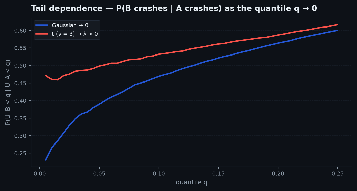
Fit a copula to the return panel — the dependence structure with the marginals stripped away. Two families: "gaussian" (no tail dependence — extremes are asymptotically independent, which is exactly the assumption that failed in 2008) and "t" (Student-t with df degrees of freedom — joint extremes cluster, and the lower df, the harder they cluster). The correlation matrix is derived from Kendall’s tau via rho = sin(pi/2 * tau), which is the correct inversion for both families.

fit_copula(returns: pd.DataFrame, family: str = "gaussian", df: float = 5.0) -> Copula

Param	Type	Default	Meaning
`returns`	pd.DataFrame	—	Per-period returns, one column per asset.
`family`	str	"gaussian"	"gaussian" or "t".
`df`	float	5.0	Degrees of freedom (t family only; lower = fatter joint tails).

Returns: a Copula dataclass with fields family, corr (a pd.DataFrame) and df.

cop_g = ek.dependence.fit_copula(rets)                       # gaussian
cop_t = ek.dependence.fit_copula(rets, family="t", df=4.0)   # tail-dependent

sample_copula#

Draw joint scenarios from a fitted copula. Gaussian: correlated normals pushed through the normal CDF. Student-t: correlated normals scaled by a shared chi-square draw, pushed through the t CDF — the sharedscale is what makes extremes arrive together. Output is uniforms; feed them to your marginals’ quantile functions to build return scenarios for stress-testing a portfolio.

sample_copula(cop: Copula, n: int, rng=None) -> pd.DataFrame

Param	Type	Default	Meaning
`cop`	Copula	—	A fitted Copula from fit_copula.
`n`	int	—	Number of joint draws.
`rng`	np.random.Generator	None	Seeded generator; defaults to bootstrap_rng().

Returns: an n x d pd.DataFrame of uniforms in (0, 1), columns matching the fitted panel. Deterministic given a seeded rng.

from edgekit.core import bootstrap_rng
u = ek.dependence.sample_copula(cop_t, n=10_000, rng=bootstrap_rng())
# map uniforms through empirical marginals to get return scenarios
scenarios = u.apply(lambda col: rets[col.name].quantile(col).to_numpy())

Tail dependence & structure#

tail_dependence#

The empirical co-crash measure: given x is in its worst q fraction of days, how often is y in its worst q too (and the mirror image for the upper tail)? Under a Gaussian copula both numbers shrink to zero as qshrinks; real equity pairs hold a stubbornly high lower value. This is the single most direct diagnostic of “my diversification will vanish when I need it”.

tail_dependence(x, y, q: float = 0.05) -> dict

Param	Type	Default	Meaning
`x`	array-like	—	Return series.
`y`	array-like	—	Return series, same length.
`q`	float	0.05	Tail fraction defining an extreme day.

Returns: a dict with keys "lower" and "upper" — conditional co-exceedance probabilities in [0, 1].

td = ek.dependence.tail_dependence(rets["SPY"], rets["EEM"], q=0.05)
td["lower"], td["upper"]   # lower >> upper for most equity pairs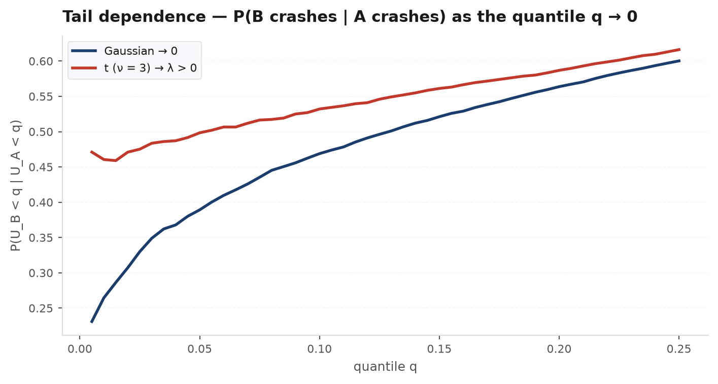

tail dependence chart — Lower vs upper tail co-exceedance — the asymmetry a Pearson number cannot see.

corr_mst#

The minimum-spanning tree of the correlation matrix (Mantegna). Correlations become distances via d = sqrt(2 * (1 - rho)), and Prim’s algorithm keeps the d - 1strongest links that connect everything — the market’s skeleton. Useful for spotting clusters, picking genuinely-distant diversifiers, and watching the tree contract when a crisis pulls everything together.

corr_mst(returns: pd.DataFrame) -> list[tuple[str, str, float]]

Param	Type	Default	Meaning
`returns`	pd.DataFrame	—	Per-period returns, one column per asset.

Returns: a list of (name_a, name_b, distance) edges — the n_assets - 1 links of the tree, where smaller distance means tighter correlation.

edges = ek.dependence.corr_mst(rets)
for a, b, d in sorted(edges, key=lambda e: e[2]):
    print(f"{a:>6} -- {b:<6}  d={d:.3f}")