edgekit.microstructure

Liquidity and trading-cost estimators that work from plain OHLCV bars — no order book, no tick feed. Effective spread (Roll, Corwin-Schultz), price impact (Amihud, Kyle’s lambda) and order-flow toxicity (VPIN). These are the numbers that decide whether an edge that exists on paper survives the act of trading it.

What's inside. tick_rule classifies trade direction from price changes and feeds the signed-volume estimators. roll_spread and corwin_schultz estimate the effective bid-ask spread from closes and high/lows respectively. amihud and kyle_lambda measure how much price a unit of volume moves. vpin tracks the buy/sell imbalance in volume time — the toxicity gauge that spikes before liquidity vanishes.

!These are estimators, not measurements

Every function here infers a hidden quantity from bar data, and each has a known failure mode: Roll returns NaNwhenever the close-to-close autocovariance is positive (trending markets), Corwin-Schultz assumes highs and lows straddle the spread, and VPIN’s bulk classification is an approximation of true signed flow. Treat them as ranking tools — is liquidity better or worse than last month, is asset A cheaper to trade than asset B — not as ground truth for a cost model.

Trade classification#

tick_rule#

The tick rule: a bar is a “buy” if price ticked up, a “sell” if it ticked down, and inherits the previous sign when the price is unchanged. Crude, but the standard first step to signed volume when you have no quote data — and the input kyle_lambda and the imbalance-bar builders use.

tick_rule(close) -> np.ndarray

Param	Type	Default	Meaning
`close`	Series or array	—	Close (or trade) prices.

Returns: an array of +1 / -1 signs, same length as the input, with zero-change bars carrying the previous sign forward.

import edgekit as ek
signs = ek.microstructure.tick_rule(bars["close"])
signed_vol = signs * bars["volume"].to_numpy()

Spread estimators#

roll_spread#

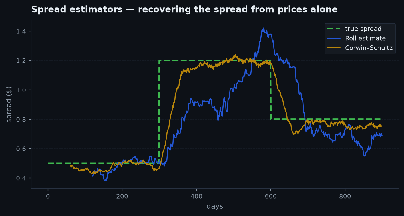
Roll (1984): if the mid-price is a random walk and trades bounce between bid and ask, the bounce induces negative autocovariance in price changes, and the effective spread is 2 * sqrt(-cov). Elegant, and honest about its limits — when the autocovariance comes out non-negative (any trending stretch), there is no spread signal in the data and you get NaN, not a made-up number.

roll_spread(close) -> float

Param	Type	Default	Meaning
`close`	Series or array	—	Close prices (use a window of recent bars).

Returns: a float — the effective spread in price units, or NaN when the price-change autocovariance is >= 0.

s = ek.microstructure.roll_spread(bars["close"].tail(250))
s / bars["close"].iloc[-1]   # as a fraction of price

corwin_schultz#

Corwin-Schultz (2012): highs and lows over one day vs two days separate volatility (grows with time) from spread (does not). Produces a spread series rather than one number, so you can watch trading cost widen into an event. Estimates are clipped at zero — the raw formula happily goes negative on quiet days.

corwin_schultz(high, low) -> pd.Series

Param	Type	Default	Meaning
`high`	Series	—	Bar highs.
`low`	Series	—	Bar lows, same index.

Returns: a pd.Series of fractional spread estimates indexed like the input, clipped at >= 0.

cs = ek.microstructure.corwin_schultz(bars["high"], bars["low"])
cs.rolling(21).mean().plot()   # monthly-smoothed effective spread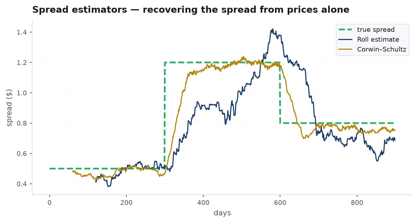

spread estimators chart — Roll and Corwin-Schultz spread estimates against a widening true spread.

Impact & illiquidity#

amihud#

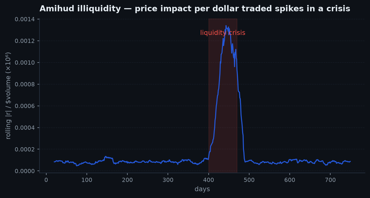
The Amihud illiquidity ratio: average absolute return per dollar of volume, on a rolling window, scaled by 1e6 to land in readable units. The workhorse cross-sectional liquidity measure — high Amihud means small flows move the price a lot, i.e. your size will cost you. Rankings from this simple ratio track sophisticated impact models remarkably well.

amihud(close, volume, window: int = 21) -> pd.Series

Param	Type	Default	Meaning
`close`	Series	—	Close prices.
`volume`	Series	—	Bar volume, same index.
`window`	int	21	Rolling window in bars.

Returns: a pd.Series — rolling mean of |r| / (close * volume), scaled by 1e6, indexed like the input.

illiq = ek.microstructure.amihud(bars["close"], bars["volume"])
illiq.iloc[-1] / illiq.median()   # >2 means liquidity has halved vs normal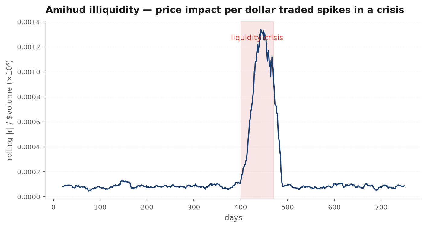

amihud illiquidity chart — Rolling Amihud illiquidity — spikes mark the stretches where size gets expensive.

kyle_lambda#

Kyle’s lambda: the slope of a rolling OLS of price changes on signed volume (signs from tick_rule). This is price impact as a regression coefficient — how many price units one unit of net order flow buys. Where Amihud is a ratio, lambda is a fitted sensitivity, and its rises flag the moments when the market stops absorbing flow.

kyle_lambda(close, volume, window: int = 63) -> pd.Series

Param	Type	Default	Meaning
`close`	Series	—	Close prices.
`volume`	Series	—	Bar volume, same index.
`window`	int	63	Rolling regression window in bars.

Returns: a pd.Series of rolling impact slopes indexed like the input (first window - 1 values NaN).

lam = ek.microstructure.kyle_lambda(bars["close"], bars["volume"])
# expected impact of trading q units in a bar: ~ lam * q

Order-flow toxicity#

vpin#

VPIN (Easley, López de Prado, O’Hara): volume-synchronised probability of informed trading. Volume is diced into equal-size buckets; each bucket’s flow is split into buy/sell via bulk volume classification — the normal CDF of the standardised price change allocates the fraction — and VPIN is the rolling average absolute imbalance. High VPIN means the flow is one-sided and market makers are being run over; it spiked hours before the 2010 flash crash.

vpin(close, volume, n_buckets: int = 50, window: int = 50) -> pd.Series

Param	Type	Default	Meaning
`close`	Series	—	Close prices.
`volume`	Series	—	Bar volume, same index.
`n_buckets`	int	50	Volume buckets the sample is diced into.
`window`	int	50	Buckets averaged into each VPIN value.

Returns: a pd.Series of VPIN values in [0, 1] (higher = more toxic flow), indexed by the bar closing each bucket.

v = ek.microstructure.vpin(bars["close"], bars["volume"])
v > v.quantile(0.95)   # the "stand aside" flag for liquidity-taking strategies