edgekit.execution

Optimal execution and transaction-cost analysis — how to trade a position, not just when. The Almgren-Chriss impact/risk trade-off, the square-root impact law, TWAP and VWAP schedules, and the implementation-shortfall decomposition that tells you where your slippage actually went.

What's inside. almgren_chriss solves the classic liquidation problem and returns an ACResult with the optimal trajectory and its cost/variance; sqrt_impact is the one-line empirical impact law; twap_schedule and vwap_schedule build the two benchmark schedules; and implementation_shortfall audits real fills against the decision price.

→Convention: quantities and costs

Schedules are in the same units as the quantity you pass in and always sum to it. Impact and shortfall numbers are fractions of price unless the name says otherwise — implementation_shortfall reports in basis points, with side=+1 for a buy and side=-1 for a sell so that a positivenumber always means “you paid”.

Optimal liquidation#

almgren_chriss#

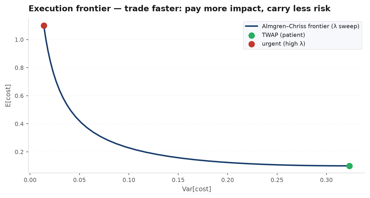
The Almgren-Chriss optimal execution trajectory. Trading fast costs impact; trading slow costs price risk; the risk-aversion lam sets the exchange rate between them. The closed-form solution decays the remaining position as x_j = x0 * sinh(kappa * (T - t_j)) / sinh(kappa * T) with urgency kappa = sqrt(lam * sigma^2 / eta): risk-neutral traders (lam → 0) get TWAP, nervous traders front-load.

@dataclass
class ACResult:
    trajectory: np.ndarray    # remaining position at each of the n+1 grid times
    expected_cost: float
    cost_variance: float
    kappa: float

almgren_chriss(x0: float, t: float, n: int, sigma: float, eta: float, lam: float) -> ACResult

Param	Type	Default	Meaning
`x0`	float	—	Initial position to liquidate (shares / contracts).
`t`	float	—	Liquidation horizon (e.g. in days).
`n`	int	—	Number of trading intervals.
`sigma`	float	—	Price volatility per unit of t (price units).
`eta`	float	—	Temporary impact coefficient (cost per unit trade rate).
`lam`	float	—	Risk aversion; 0 = TWAP, larger = more front-loaded.

Returns: an ACResult — trajectory (length n + 1, from x0 down to 0), expected_cost, cost_variance and the urgency kappa.

import edgekit as ek
res = ek.execution.almgren_chriss(x0=100_000, t=1.0, n=13, sigma=0.4, eta=2.5e-6, lam=2e-6)
res.trajectory        # holdings at each interval boundary
-np.diff(res.trajectory)   # shares to trade in each interval
res.expected_cost, res.cost_variance

Sweep lam and plot expected_cost vs sqrt(cost_variance) to trace the efficient frontier of execution — every point on it is optimal for some risk appetite; everything above it is just bad trading.

Almgren-Chriss frontier chart — The execution frontier: expected cost against cost risk as lam sweeps from patient to urgent.

Impact#

sqrt_impact#

The square-root law — the most robust empirical regularity in market impact: trading q against average daily volume adv moves the price about c * sigma_daily * sqrt(q / adv). Concave, so the second block of a big order is cheaper than the first — and brutal on capacity, because impact grows with the square root of size while your edge does not grow at all.

sqrt_impact(q: float, adv: float, sigma_daily: float, c: float = 1.0) -> float

Param	Type	Default	Meaning
`q`	float	—	Order size (same units as adv).
`adv`	float	—	Average daily volume.
`sigma_daily`	float	—	Daily return volatility (fraction).
`c`	float	1.0	Impact coefficient (empirically ~0.5–1.5).

Returns: a float — expected impact as a fraction of price.

imp = ek.execution.sqrt_impact(q=50_000, adv=2_000_000, sigma_daily=0.02)
imp * 1e4    # in basis points; compare against your per-trade edge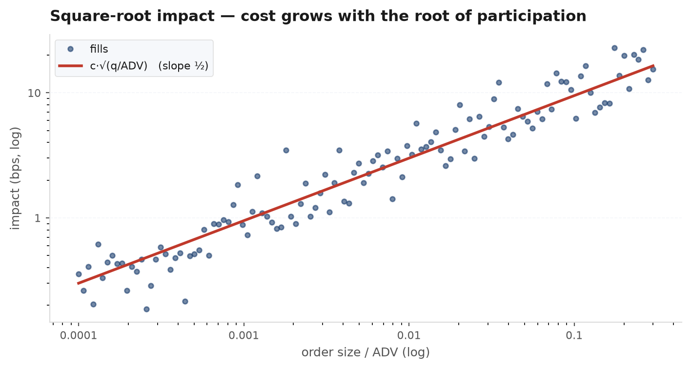

square-root impact chart — Impact vs participation: the square-root law's concave bite out of a fixed per-trade edge.

Benchmark schedules#

twap_schedule#

Time-weighted average price: the quantity split into n equal slices. The zero-information benchmark — also the Almgren-Chriss optimum when risk aversion is zero. If a clever schedule cannot beat TWAP after costs, trade TWAP.

twap_schedule(qty: float, n: int) -> np.ndarray

Param	Type	Default	Meaning
`qty`	float	—	Total quantity to trade.
`n`	int	—	Number of slices.

Returns: a length-n array of equal slices summing to qty.

slices = ek.execution.twap_schedule(10_000, n=8)   # eight lots of 1250

vwap_schedule#

Volume-weighted: slices proportional to an expected intraday volume profile, so you trade heavily when the market does (open and close) and lightly through the lunchtime trough — holding your participation rate, and hence your impact, roughly constant.

vwap_schedule(qty: float, volume_profile) -> np.ndarray

Param	Type	Default	Meaning
`qty`	float	—	Total quantity to trade.
`volume_profile`	array-like	—	Expected volume per interval (any positive scale).

Returns: an array the length of the profile, proportional to it and summing to qty.

profile = bars.groupby(bars.index.time)["volume"].mean()   # historical U-shape
slices = ek.execution.vwap_schedule(10_000, profile.to_numpy())

Post-trade analysis#

implementation_shortfall#

Perold’s implementation shortfall: the all-in gap between the price when you decided and what you actually achieved, decomposed into delay cost (decision → arrival, the price drifting away while you hesitated) and execution cost (arrival → fills, the impact and spread you paid while working). The number your backtest silently assumed was zero.

implementation_shortfall(decision_price, fill_prices, fill_qtys, side: int = 1,
                         arrival_price: float | None = None) -> dict

Param	Type	Default	Meaning
`decision_price`	float	—	Price when the trade decision was made.
`fill_prices`	array-like	—	Price of each fill.
`fill_qtys`	array-like	—	Quantity of each fill.
`side`	int	1	+1 buy, -1 sell (positive output = cost either way).
`arrival_price`	float \| None	None	Price when the order hit the market; enables the delay split.

Returns: a dict with "total_bps", "delay_bps", "execution_bps" and "avg_fill" (the quantity-weighted average fill price).

out = ek.execution.implementation_shortfall(
    decision_price=101.20, fill_prices=[101.32, 101.38, 101.45],
    fill_qtys=[400, 400, 200], side=+1, arrival_price=101.28)
out["total_bps"], out["delay_bps"], out["execution_bps"]
# chronic delay_bps: your signal is decaying before you act
# chronic execution_bps: you are trading too fast for the book

!Close the loop with the backtest

The point of TCA is comparison: total_bps, averaged over live trades, should match the cost your backtest charged per trade. If live shortfall runs at 9 bps and your backtest assumed 3, every backtested metric is wrong by the difference — re-run the cost-stressstep with reality’s number before trusting anything else.