edgekit.sim

One home for path simulation — GBM, jumps, stochastic vol, GARCH and regime-switching — plus the variance-reduction and quasi-random machinery that makes Monte Carlo answers arrive sooner. Every stochastic function takes an rng and defaults to the library-wide bootstrap_rng(), so every simulation in edgekit is reproducible given a seed.

What's inside. Three price-path models — gbm_paths (the baseline), merton_paths (adds jumps), heston_paths (adds stochastic volatility) — and two return-path models, garch_paths (volatility clustering) and regime_switching_paths (calm/panic states). Then the tools that sharpen any of them: antithetic and control_variate for variance reduction, halton and quasi_normals for low-discrepancy sampling.

→Convention: shapes and seeding

Price-path functions return arrays of shape (n_paths, steps + 1) — row 0 of every path is s0. Return-path functions return (n_paths, n) per-period returns. Pass rng=bootstrap_rng(seed) to make any run repeatable; omit it and you get the library default seed, so two calls in the same session still agree.

Price paths#

gbm_paths#

Geometric Brownian motion — the Black-Scholes world. Constant drift, constant volatility, lognormal terminal prices. Wrong in every interesting way (no fat tails, no clustering, no jumps), which is precisely why it is the baseline: anything your strategy does on GBM paths it does by construction, not by edge.

gbm_paths(s0, mu, sigma, t=1.0, steps=252, n_paths=1000, rng=None) -> np.ndarray

Param	Type	Default	Meaning
`s0`	float	—	Starting price.
`mu`	float	—	Annualised drift.
`sigma`	float	—	Annualised volatility.
`t`	float	1.0	Horizon in years.
`steps`	int	252	Time steps over the horizon.
`n_paths`	int	1000	Number of paths.
`rng`	np.random.Generator	None	Seeded generator; defaults to bootstrap_rng().

Returns: an (n_paths, steps + 1) array of prices.

import edgekit as ek
from edgekit.core import bootstrap_rng
S = ek.sim.gbm_paths(100.0, mu=0.07, sigma=0.2, rng=bootstrap_rng())
S[:, -1].mean()   # ~ 100 * exp(0.07)

merton_paths#

GBM plus a compound-Poisson jump component (Merton 1976). Jumps arrive at rate lam per year with lognormal sizes — the model that admits crashes are a thing that happens between ticks, not a large diffusion move. The one to use when you want gap risk in a stop-loss study.

merton_paths(s0, mu, sigma, lam, jump_mu, jump_sigma,
             t=1.0, steps=252, n_paths=1000, rng=None) -> np.ndarray

Param	Type	Default	Meaning
`s0, mu, sigma`	float	—	As in gbm_paths (diffusion part).
`lam`	float	—	Jump intensity — expected jumps per year.
`jump_mu`	float	—	Mean log jump size (negative for crash-like jumps).
`jump_sigma`	float	—	Std of log jump size.
`t / steps / n_paths / rng`	—	1.0 / 252 / 1000 / None	As in gbm_paths.

Returns: an (n_paths, steps + 1) array of prices.

S = ek.sim.merton_paths(100.0, mu=0.07, sigma=0.15,
                        lam=1.0, jump_mu=-0.08, jump_sigma=0.05)  # ~1 crash/yr

heston_paths#

The Heston stochastic-volatility model: variance itself follows a mean-reverting square-root process, correlated with returns via rho (negative rho = the leverage effect — vol spikes when prices fall). Discretised with the full-truncation Euler scheme, the standard fix that keeps variance from going negative without biasing the drift.

heston_paths(s0, mu, v0, kappa, theta, xi, rho,
             t=1.0, steps=252, n_paths=1000, rng=None) -> tuple[np.ndarray, np.ndarray]

Param	Type	Default	Meaning
`s0, mu`	float	—	Starting price and annualised drift.
`v0`	float	—	Starting variance (vol squared).
`kappa`	float	—	Mean-reversion speed of variance.
`theta`	float	—	Long-run variance level.
`xi`	float	—	Vol-of-vol.
`rho`	float	—	Return–variance correlation (typically negative).
`t / steps / n_paths / rng`	—	1.0 / 252 / 1000 / None	As in gbm_paths.

Returns: a tuple (S, V) — prices and variance paths, each (n_paths, steps + 1).

S, V = ek.sim.heston_paths(100.0, mu=0.05, v0=0.04, kappa=2.0,
                           theta=0.04, xi=0.5, rho=-0.7)
np.sqrt(V[:, -1]).mean()   # terminal vol hovers near sqrt(theta)

Return paths#

garch_paths#

Simulate GARCH(1,1) return paths — the model that reproduces volatility clustering: big days follow big days. Use these paths to test anything that conditions on realised vol (vol targeting, ATR stops) against a world where quiet and violent stretches alternate the way real markets do.

garch_paths(mu, omega, alpha, beta, n=1000, n_paths=100, rng=None) -> np.ndarray

Param	Type	Default	Meaning
`mu`	float	—	Per-period mean return.
`omega`	float	—	Baseline variance constant.
`alpha`	float	—	Reaction to yesterday's shock.
`beta`	float	—	Persistence of yesterday's variance (alpha + beta < 1).
`n`	int	1000	Periods per path.
`n_paths`	int	100	Number of paths.
`rng`	np.random.Generator	None	Seeded generator.

Returns: an (n_paths, n) array of per-period returns.

# feed fitted params straight back in
fit = ek.timeseries.garch11(rets)
R = ek.sim.garch_paths(mu=0.0, omega=fit["omega"], alpha=fit["alpha"], beta=fit["beta"])

regime_switching_paths#

A two-state Markov world: a calm regime (small positive drift, low vol) and a panic regime (negative drift, high vol), with sticky transition probabilities. The defaults are deliberately equity-like. Returns both the return paths and the hidden state matrix, so you can score a regime detector against the truth it never gets to see in real data.

regime_switching_paths(mu=(0.0008, -0.0005), sigma=(0.008, 0.025),
                       p_stay=(0.98, 0.95), n=1000, n_paths=100, rng=None)
    -> tuple[np.ndarray, np.ndarray]

Param	Type	Default	Meaning
`mu`	tuple	(0.0008, -0.0005)	Per-period drift in (calm, panic).
`sigma`	tuple	(0.008, 0.025)	Per-period vol in (calm, panic).
`p_stay`	tuple	(0.98, 0.95)	Probability of remaining in each state.
`n / n_paths / rng`	—	1000 / 100 / None	Periods, paths, generator.

Returns: a tuple (returns, states) — both (n_paths, n); states holds 0 (calm) / 1 (panic).

R, Z = ek.sim.regime_switching_paths(n=2000, n_paths=50)
R[Z == 1].std() / R[Z == 0].std()   # ~3x vol ratio between regimes

Variance reduction#

antithetic#

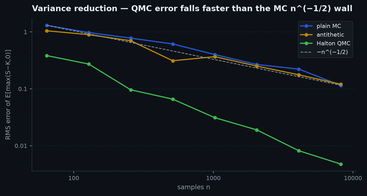
Antithetic normals: draw half the sample, mirror it. Every draw z is paired with -z, so odd-moment sampling error cancels exactly and smooth-payoff estimates tighten at zero extra cost. Feed these into any path builder in place of raw normals.

antithetic(n: int, d: int = 1, rng=None) -> np.ndarray

Param	Type	Default	Meaning
`n`	int	—	Total draws (second half is the negation of the first).
`d`	int	1	Dimensions per draw.
`rng`	np.random.Generator	None	Seeded generator.

Returns: an (n, d) array of standard normals with exact mirror symmetry.

z = ek.sim.antithetic(10_000)
z.mean()   # exactly 0.0 by construction

control_variate#

The control-variate estimator: you want E[y], you also simulated x whose true mean you know (a GBM terminal price, a vanilla option under Black-Scholes). Regress y on x and subtract the known error — the variance drops by the squared correlation between them.

control_variate(y, x, x_true_mean) -> dict

Param	Type	Default	Meaning
`y`	array-like	—	Simulated values of the target quantity.
`x`	array-like	—	Simulated control, same draws / same length.
`x_true_mean`	float	—	The control's exact analytic mean.

Returns: a dict with "estimate" (the corrected mean), "beta" (the regression coefficient) and "var_reduction" (variance ratio vs the naive mean).

# price an exotic using the vanilla as control
out = ek.sim.control_variate(exotic_payoffs, vanilla_payoffs, x_true_mean=bs_price)
out["estimate"], out["var_reduction"]   # e.g. 5-20x fewer paths needed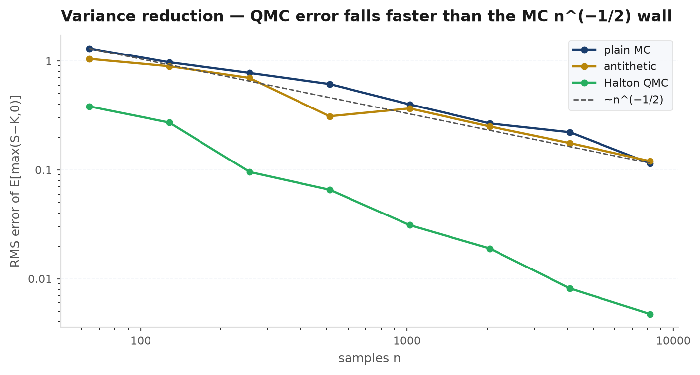

variance reduction chart — Naive vs antithetic vs control-variate estimator error at the same path budget.

Quasi-random sequences#

halton#

The Halton low-discrepancy sequence — deterministic points that fill the unit cube far more evenly than random draws, using the first d primes as bases. Integration error shrinks near 1/n instead of 1/sqrt(n) in low dimensions. No rng: the sequence is the same every time, by design.

halton(n: int, d: int = 1) -> np.ndarray

Param	Type	Default	Meaning
`n`	int	—	Number of points.
`d`	int	1	Dimensions (first d primes as bases; keep d modest).

Returns: an (n, d) array of points in (0, 1).

u = ek.sim.halton(1024, d=2)   # evenly-spread pairs, no clumps

quasi_normals#

Halton points mapped through the inverse normal CDF (the same Acklam _norm_ppf the risk module uses) — quasi-random standard normals, ready to drive a path simulation with low-discrepancy shocks instead of pseudo-random ones.

quasi_normals(n: int, d: int = 1) -> np.ndarray

Param	Type	Default	Meaning
`n`	int	—	Number of draws.
`d`	int	1	Dimensions.

Returns: an (n, d) array of deterministic quasi-normal draws.

z = ek.sim.quasi_normals(4096)
z.mean(), z.std()   # ~0, ~1 — but far smoother tails coverage than pseudo-random