Markov chains

A Markov chain is a random process with amnesia: given the present state, the future is independent of the past. That one assumption buys an enormous amount of machinery — transition matrices, stationary distributions, and above all first-step analysis, the single most-used tool in applied probability. This chapter builds the theory, then drills the tool on the classics: expected flips to HH versus HT, frogs, mazes, deuce, and a drunk near a cliff.

✦Intuition — why memorylessness is a feature, not a bug

Most real systems have long memories, but a surprising number are well described by a handful of stateswhose label absorbs everything relevant about the past: the weather is “wet” or “dry”, the market is “calm” or “turbulent”, your coin-flip progress toward HH is “nothing yet” or “one head”. Once the state summarises the past, the process restarts from the state — and every question about the future becomes linear algebra. That is the whole trick: choose the state so the process forgets, then condition on one step.

The Markov property and transition matrices#

A discrete-time process $(X_{n})_{n \geq 0}$ on a countable state space $S$ is a Markov chain if for all states and all $n$ ,

P (X_{n + 1} = j ∣ X_{n} = i, X_{n - 1} = i_{n - 1}, \dots, X_{0} = i_{0}) = P (X_{n + 1} = j ∣ X_{n} = i) = p_{ij} .

The chain is time-homogeneous when $p_{ij}$ does not depend on $n$ . Collect the one-step probabilities into the transition matrix $P = (p_{ij})$ : every entry is non-negative and every row sums to one (a stochastic matrix). If the distribution of $X_{n}$ is the row vector $μ_{n}$ , then $μ_{n + 1} = μ_{n} P$ — the entire dynamics is matrix multiplication.

A running example with a quant flavour: a two-state regime chain for daily market conditions, calm (C) or turbulent (T),

P = (0.95 0.20 0.05 0.80) rows/columns ordered (C, T) .

Calm days overwhelmingly stay calm; turbulence persists but decays. This is exactly the structure behind regime detection — a hidden Markov model is this chain with noisy observations bolted on.

✦Proof — Chapman–Kolmogorov and n-step transitions

Write $p_{ij}^{(n)} = P (X_{n} = j ∣ X_{0} = i)$ . Condition on the state at an intermediate time $m$ using the law of total probability (see axioms & conditioning) and apply the Markov property to drop the past:

p_{ij}^{(m + n)} = k \in S \sum P (X_{m} = k ∣ X_{0} = i) P (X_{m + n} = j ∣ X_{m} = k) = k \in S \sum p_{ik}^{(m)} p_{k j}^{(n)} .

But the right side is precisely the $(i, j)$ entry of the matrix product $P^{m} P^{n}$ . By induction the $n$ -step transition matrix is $P^{(n)} = P^{n}$ : powers of the one-step matrix. Every multi-step question about a Markov chain is a statement about matrix powers.

Worked example (by hand). Starting calm, what is the probability of turbulence two days out? Sum over the intermediate day:

p_{C T}^{(2)} = p_{C C} p_{C T} + p_{C T} p_{T T} = 0.95 \times 0.05 + 0.05 \times 0.80 = 0.0475 + 0.04 = 0.0875.

Either you stay calm a day and then flip, or you flip immediately and turbulence persists. Note $0.0875 > 0.05$ : risk accumulates with horizon, but not linearly — the two-step matrix is already blending toward the long-run mix computed below.

Classifying states#

The long-run behaviour of a chain is controlled by a small taxonomy. State $j$ is accessible from $i$ if $p_{ij}^{(n)} > 0$ for some $n$ ; states that access each other communicate, and a chain whose states all communicate is irreducible.

Recurrent: starting from $i$ , the chain returns to $i$ with probability 1 (and hence infinitely often). If the expected return time is finite the state is positive recurrent.
Transient: the return probability is $< 1$ ; the chain visits the state only finitely many times, then leaves forever. Equivalent test: $\sum_{n} p_{ii}^{(n)} < \infty$ .
Periodic: the period of $i$ is $d (i) = g cd {n : p_{ii}^{(n)} > 0}$ . A chain that can only return at even times (period 2, like the simple random walk) never settles pointwise — it oscillates. Aperiodic means $d (i) = 1$ .
Absorbing: $p_{ii} = 1$ — once entered, never left. Ruin at zero wealth is the canonical example.

In a finite chain, at least one state must be recurrent (the chain has nowhere else to go), and all states of an irreducible finite chain are positive recurrent. Transience only truly bites on infinite state spaces — the random walk in three dimensions is the famous example, taken up in random walks & Brownian motion.

Stationary distributions and convergence#

A distribution $π$ (a row vector, $π_{i} \geq 0$ , $\sum_{i} π_{i} = 1$ ) is stationary if it is a fixed point of the dynamics:

π P = π ⟺ π_{j} = i \sum π_{i} p_{ij} for all j .

Start the chain in $π$ and it stays in $π$ forever. The fundamental theorem for finite chains: if the chain is irreducible, a stationary distribution exists and is unique, and $π_{i} = 1/ E_{i} [return time to i]$ . If additionally the chain is aperiodic, then from any start,

p_{ij}^{(n)} ⟶ π_{j} as n \to \infty,

and long-run time averages converge to $π$ -averages (the ergodic theorem — the Markov cousin of the law of large numbers).

Worked example (by hand). Solve $π P = π$ for the regime chain. With $π = (π_{C}, π_{T})$ , the balance equation for state C reads $π_{C} = 0.95 π_{C} + 0.20 π_{T}$ , i.e. $0.05 π_{C} = 0.20 π_{T}$ . Probability out of calm must match probability into calm. With $π_{C} + π_{T} = 1$ :

π_{C} = \frac{0.20}{0.20 + 0.05} = 0.8, π_{T} = 0.2.

The market spends 80% of days calm in the long run, and the expected return time to turbulence is $1/ π_{T} = 5$ days. The general two-state shortcut is worth memorising: with switch probabilities $a$ (out of state 1) and $b$ (out of state 2), $π = (\frac{b}{a + b}, \frac{a}{a + b})$ .

✦Proof — detailed balance implies stationarity

A distribution $π$ satisfies detailed balance if $π_{i} p_{ij} = π_{j} p_{j i}$ for every pair — probability flows between each pair of states in equal and opposite amounts. Summing over $i$ :

i \sum π_{i} p_{ij} = i \sum π_{j} p_{j i} = π_{j} i \sum p_{j i} = π_{j},

which is exactly $π P = π$ . Detailed balance is stronger than stationarity (it makes the chain look statistically identical run backwards — reversible), but it is much easier to solve: pairwise equations instead of a global linear system. Every two-state chain is reversible — check ours: $π_{C} p_{C T} = 0.8 \times 0.05 = 0.04 = 0.2 \times 0.20 = π_{T} p_{T C}$ . This is also the design principle behind MCMC samplers: build $P$ to satisfy detailed balance with respect to the distribution you want to sample.

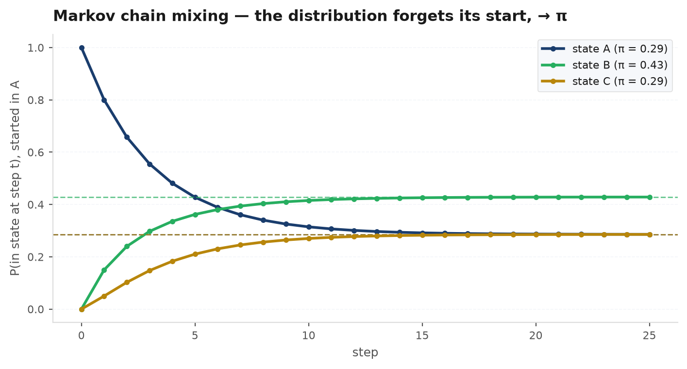
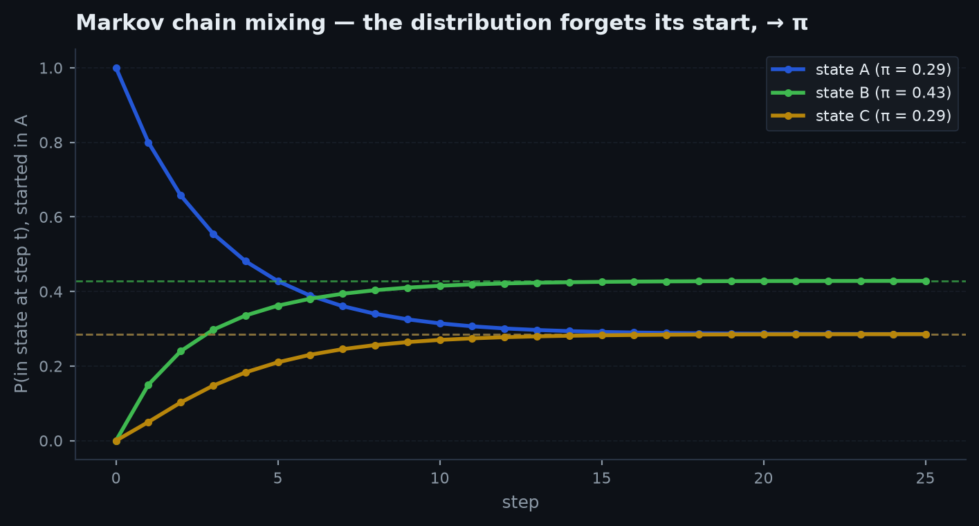
Rows of the n-step transition matrix of a two-state chain converging geometrically to the stationary distribution from different starting states — Convergence to stationarity: the probability of being turbulent after n days, started calm versus started turbulent. Both curves converge geometrically to pi_T = 0.2 at rate |lambda_2| = 0.75 per step — the second eigenvalue of P sets the mixing speed, and the starting state is forgotten.

The speed of convergence is geometric, governed by the second-largest eigenvalue modulus of $P$ (here $λ_{2} = 0.95 + 0.80 - 1 = 0.75$ ): distance to stationarity shrinks by a factor $∣ λ_{2} ∣$ per step. Slow mixing (eigenvalue near 1) means persistent regimes — the statistical reason regime filters lag turns.

→Quant lens — regimes, persistence, and why sample averages mislead

Markov-chain persistence is the simplest model of volatility clustering: conditional on today being turbulent, tomorrow is turbulent with 0.80, not the unconditional 0.2. Two consequences for practice. First, unconditional statistics (average vol, average correlation) blend regimes and describe no actual market day — condition on state, as in regime detection. Second, persistence slashes the effective sample size of a backtest: 1,000 daily observations of a slowly mixing chain carry far fewer independent data points than 1,000 coin flips, exactly the autocorrelation penalty derived in LLN & CLT.

markov_sim.py

import numpy as np

rng = np.random.default_rng(11)
P = np.array([[0.95, 0.05],
              [0.20, 0.80]])          # states: 0 = calm, 1 = turbulent

# --- 1) long-run occupation matches pi = (0.8, 0.2) ---------------------
n, x = 200_000, 0
visits = np.zeros(2)
for _ in range(n):
    visits[x] += 1
    x = rng.choice(2, p=P[x])
print(visits / n)                     # ~ [0.800, 0.200]

# eigenvector check: left eigenvector of P for eigenvalue 1
w, V = np.linalg.eig(P.T)
pi = np.real(V[:, np.argmax(w)]); pi /= pi.sum()
print(pi)                             # [0.8, 0.2]

# --- 2) first-step analysis check: expected fair flips to see HH = 6 ----
def flips_to_HH():
    prev, t = None, 0
    while True:
        c = rng.integers(2); t += 1   # 1 = heads
        if prev == 1 and c == 1:
            return t
        prev = c
print(np.mean([flips_to_HH() for _ in range(200_000)]))  # ~ 6.0

First-step analysis: the essential tool#

Almost every Markov problem — hitting probabilities, expected durations, win probabilities from a score — yields to one move: condition on the first step. Let $A \subset S$ be a target set. Define the hitting probability $h_{i} = P_{i} (hit A)$ and the expected hitting time $k_{i} = E_{i} [steps to reach A]$ . Conditioning on $X_{1}$ and using the Markov property to restart the chain gives linear systems:

h_{i} = j \sum p_{ij} h_{j} (i \in / A), h_{i} = 1 (i \in A);

k_{i} = 1 + j \sum p_{ij} k_{j} (i \in / A), k_{i} = 0 (i \in A) .

Read the second system aloud and it is obvious: one step happens no matter what, plus wherever you land, you face the same problem from the new state. The boundary conditions do the rest. (When several solutions exist — possible on infinite spaces — the hitting probabilities are the minimal non-negative solution.)

Worked example 1 — hitting probability. A fair gambler starts with 1 unit and quits at 0 (broke) or 3 (target); each round is $\pm 1$ with probability $1/2$ . Let $h_{i}$ be the probability of reaching 3 from $i$ . Boundaries $h_{0} = 0$ , $h_{3} = 1$ ; interior:

h_{1} = \frac{1}{2} h_{0} + \frac{1}{2} h_{2}, h_{2} = \frac{1}{2} h_{1} + \frac{1}{2} h_{3} .

Substituting: $h_{1} = \frac{1}{2} (\frac{1}{2} h_{1} + \frac{1}{2}) = \frac{1}{4} h_{1} + \frac{1}{4}$ , so $h_{1} = 1/3$ and $h_{2} = 2/3$ — in general $h_{i} = i / N$ for a fair game, linear in wealth. The full gambler’s-ruin treatment, including the biased case and expected duration via optional stopping, is in martingales & optional stopping — first-step analysis and martingale arguments are two roads to the same linear systems.

Worked example 2 — expected hitting time. Expected rolls of a fair die to see two consecutive sixes. States: $S$ (no progress) and $F$ (last roll was a six). Let $x_{S}, x_{F}$ be expected remaining rolls:

x_{S} = 1 + \frac{5}{6} x_{S} + \frac{1}{6} x_{F}, x_{F} = 1 + \frac{5}{6} x_{S} + \frac{1}{6} \cdot 0.

The first equation gives $x_{S} = 6 + x_{F}$ ; substituting the second, $x_{S} = 7 + \frac{5}{6} x_{S}$ , so $x_{S} = 42$ . Six rolls to get one six, but 42 to get two in a row — failure late in the pattern throws you all the way back to the start, and that resetting is expensive. This asymmetry is the heart of Problem 1 below.

Bar chart of expected hitting times from each state of a small chain, computed from the first-step linear system and matched by simulation — Expected hitting times solve a linear system: one step plus the expectation from wherever you land. The bars show the exact solution of the first-step equations; the dots are seeded simulation averages. Patterns that reset on failure (like HH, or double sixes) have much longer waits than their probability alone suggests.

Absorbing chains and the fundamental matrix#

First-step analysis scales to any number of states by matrix algebra. Order states with the transient ones first and write the transition matrix in canonical block form:

P = (Q 0 R I),

where $Q$ maps transient to transient and $R$ transient to absorbing. The fundamental matrix is $N = (I - Q)^{- 1} = I + Q + Q^{2} + \dots$ : entry $N_{ij}$ is the expected number of visits to transient state $j$ starting from $i$ (each power of $Q$ counts visits at one time step). Then expected absorption times and absorption probabilities come out in one line each:

t = N 1 (expected steps to absorption), B = N R (B_{ik} = P_{i} (absorbed in k)) .

Worked example (by hand). The gambler’s chain on ${0, 1, 2, 3}$ has transient states ${1, 2}$ with

Q = (0 \frac{1}{2} \frac{1}{2} 0), N = (I - Q)^{- 1} = \frac{1}{1 - \frac{1}{4}} (1 \frac{1}{2} \frac{1}{2} 1) = (\frac{4}{3} \frac{2}{3} \frac{2}{3} \frac{4}{3}) .

So $t = N 1 = (2, 2)^{⊤}$ — two expected rounds from either interior state (matching the general fair-game formula $i (N - i) = 1 \times 2$ ) — and $B = N R$ reproduces $h_{1} = 1/3, h_{2} = 2/3$ from the previous section. One matrix inverse answers every hitting question about the chain at once.

Practice problems#

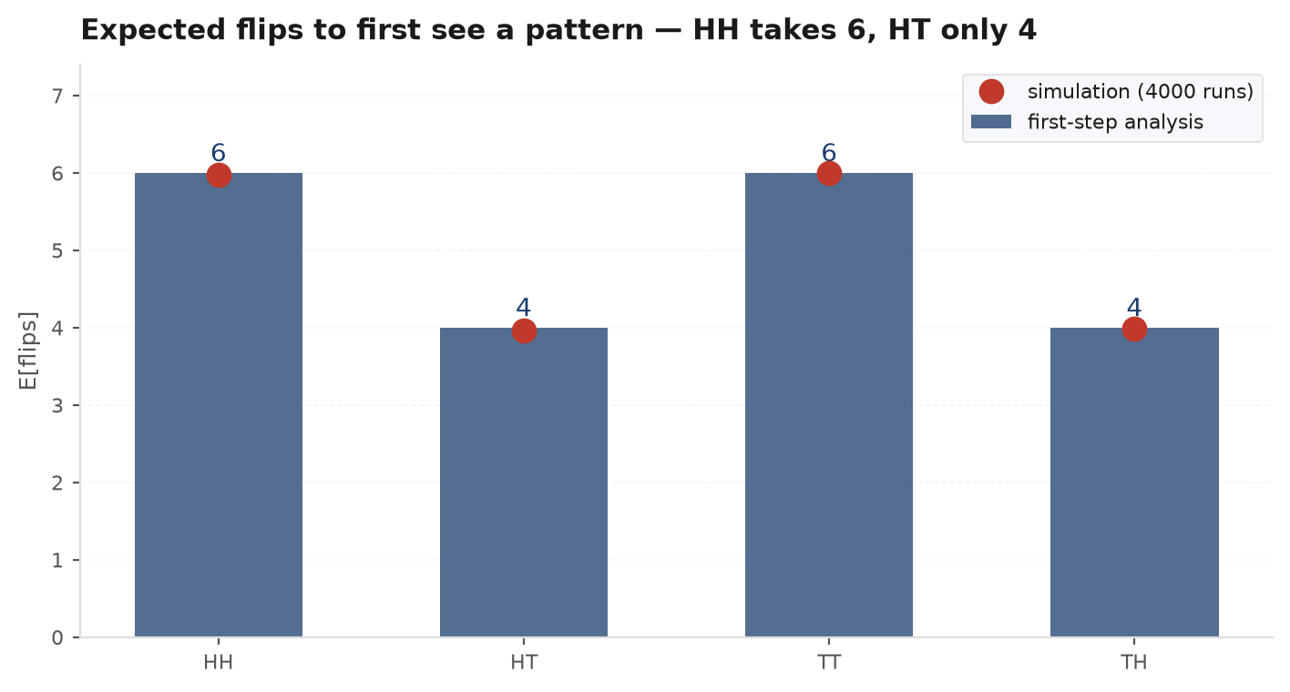
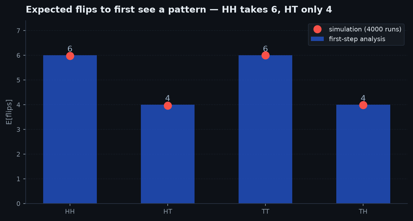
→Problem 1 — Expected flips: HH versus HT

A fair coin is flipped until the pattern HH first appears; separately, until HT first appears. Find both expected waiting times and explain why they differ.

Solution. HH. Track progress with states $S_{0}$ (no useful history) and $S_{H}$ (last flip H, no HH yet). First-step equations for the expected remaining flips $x_{0}, x_{H}$ :

x_{0} = 1 + \frac{1}{2} x_{H} + \frac{1}{2} x_{0}, x_{H} = 1 + \frac{1}{2} \cdot 0 + \frac{1}{2} x_{0} .

From the first, $x_{0} = 2 + x_{H}$ . Substitute the second: $x_{0} = 3 + \frac{1}{2} x_{0}$ , hence $x_{0} = 6$ (and $x_{H} = 4$ ).

HT. Same states, but now from $S_{H}$ a head is not a setback — it leaves you still holding a head:

y_{0} = 1 + \frac{1}{2} y_{H} + \frac{1}{2} y_{0}, y_{H} = 1 + \frac{1}{2} \cdot 0 + \frac{1}{2} y_{H} .

The second equation solves alone: $y_{H} = 2$ ; then $y_{0} = 2 + y_{H} =$ $4$ .

Why they differ. Both patterns occur with the same probability $1/4$ in any two given flips, but the failure geometry differs. Waiting for HH, a tail after a head destroys all progress — back to $S_{0}$ . Waiting for HT, once you hold a head you can never lose it: extra heads keep you at $S_{H}$ , and the first tail finishes. Equivalently, HH can overlap with itself (occurrences can share a flip), which forces occurrences to clump and stretches the mean gap between them; the general statement is the pattern-overlap (Conway leading-number) correction, and the elegant martingale proof of it is the ABRACADABRA argument in martingales & optional stopping. A classic follow-up: “so which pattern appears firstmore often?” — for HH vs HT it is a tie by symmetry of the first two outcomes, which is a different question than the mean wait.

→Problem 2 — Frog on three lily pads

A frog sits on one of three lily pads arranged in a triangle. Each minute it jumps to one of the other two pads uniformly at random. What is the expected time until it first returns to its starting pad?

Solution. Slick route: the chain is irreducible on 3 states and symmetric, so the stationary distribution is uniform, $π_{i} = 1/3$ . By the return-time theorem, $E_{i} [return time] = 1/ π_{i} = 3$ . Systematic route (first-step): from either non-start pad, let $h$ be the expected time to reach the start; by symmetry both non-start pads share it: $h = 1 + \frac{1}{2} \cdot 0 + \frac{1}{2} h$ , so $h = 2$ , and the return time is $1 + h = 3$ . The $1/ π$ shortcut is worth volunteering: it dispatches every “expected return time on a symmetric graph” variant (a knight on a chessboard corner is the famous one — return time $= total degree / corner degree = 336/2 = 168$ , since the random walk on a graph has $π_{v} \propto de g v$ by detailed balance).

→Problem 3 — Rat in a maze (three doors)

A rat is in a chamber with three doors, chosen uniformly at random each attempt. Door 1 leads outside after a 2-minute tunnel. Door 2 returns it to the chamber after 3 minutes; door 3 returns it after 5 minutes. Expected time to get out?

Solution. Let $T$ be the escape time and condition on the first choice; by the Markov property the rat restarts fresh after a returning tunnel (it learns nothing):

E [T] = \frac{1}{3} (2) + \frac{1}{3} (3 + E [T]) + \frac{1}{3} (5 + E [T]) = \frac{10}{3} + \frac{2}{3} E [T],

so $\frac{1}{3} E [T] = \frac{10}{3}$ and $E [T] = 10$ minutes. Sanity check via a renewal view: each attempt costs on average $(2 + 3 + 5) /3 = 10/3$ minutes and succeeds with probability $1/3$ , so the expected number of attempts is 3 and $3 \times 10/3 = 10$ . The trap variant gives the rat memory (it never repeats a door); then the conditioning changes and the answer drops — always ask whether the process resets.

→Problem 4 — Tennis from deuce

From deuce, a server wins each point independently with probability $p$ . A player must lead by two points to take the game. What is the probability the server wins from deuce, and the value for $p = 0.6$ ?

Solution. States: deuce $D$ , advantage-server $A$ , advantage-receiver $B$ . With $q = 1 - p$ and $w$ the win probability from deuce:

w = p w_{A} + q w_{B}, w_{A} = p + q w, w_{B} = p w .

w = p (p + q w) + q (pw) = p^{2} + 2 pq w ⟹ w = \frac{p ^{2}}{1 - 2 pq} = \frac{p ^{2}}{p ^{2} + q ^{2}} .

The slick reading: play points in pairs. A pair is decisive only if it splits $pp$ or $q q$ ; conditional on a decisive pair, the server wins with probability $p^{2} / (p^{2} + q^{2})$ , and indecisive pairs (probability $2 pq$ ) return to deuce — memorylessness makes them irrelevant. For $p = 0.6$ : $w = 0.36/ (0.36 + 0.16) = 9/13 \approx 0.692$ — a 60% point edge compounds to a 69% game edge from deuce. Expected number of points from deuce is $2/ (p^{2} + q^{2}) = 2/0.52 \approx 3.85$ (geometric number of pairs times two).

→Problem 5 — Drunk on a cliff

A drunk stands one step from a cliff edge. Each second he steps toward the edge with probability $1/3$ and away with probability $2/3$ . What is the probability he eventually falls off?

Solution. Let $q_{k}$ be the probability of ever reaching the edge from $k$ steps away. Homogeneity plus the strong Markov property give the multiplicative structure $q_{k} = q_{1}^{k}$ : to fall from distance 2 you must first reach distance 1, then fall from there, and the two stages are independent replicas. First-step analysis at $k = 1$ :

q_{1} = \frac{1}{3} + \frac{2}{3} q_{2} = \frac{1}{3} + \frac{2}{3} q_{1}^{2} ⟹ 2 q_{1}^{2} - 3 q_{1} + 1 = 0 ⟹ q_{1} \in {\frac{1}{2}, 1} .

Hitting probabilities are the minimal non-negative solution, so $q_{1} = 1/2$ . In general, stepping toward doom with probability $p < 1/2$ gives $q_{1} = p / (1 - p)$ ; at $p = 1/2$ the answer jumps to 1 — the fair walk is recurrent (see random walks), so even a fair game against a barrier is eventually fatal. That discontinuity at $p = 1/2$ is the point worth dwelling on.

→Problem 6 — Weather chain

If it rains today it rains tomorrow with probability 0.7; if it is sunny it rains tomorrow with probability 0.4. (a) Given rain today, the probability of rain the day after tomorrow? (b) The long-run fraction of rainy days?

Solution. (a) Chapman–Kolmogorov, summing over tomorrow: $p_{R R}^{(2)} = 0.7 \times 0.7 + 0.3 \times 0.4 = 0.49 + 0.12 = 0.61$ . (b) Balance flow between states: $π_{R} \times 0.3 = π_{S} \times 0.4$ , so $π_{R} = 0.4/ (0.4 + 0.3) = 4/7 \approx 0.571$ . Note the two-step answer 0.61 is already drifting from 0.7 toward the stationary 0.571 at geometric rate $λ_{2} = 0.7 - 0.4 = 0.3$ per day: after $n$ days, $p_{R R}^{(n)} = \frac{4}{7} + \frac{3}{7} (0.3)^{n}$ — a closed form worth quoting to close the question.

Next:the drunk near a cliff was a preview; the next chapter gives gambler’s ruin its own full treatment — solved three ways, by difference equations, martingales, and symmetry — and follows the consequences all the way to risk of ruin. Gambler’s ruin & fair games.